Classical simulability, entanglement breaking, and quantum computation thresholds
Abstract
We investigate the amount of noise required to turn a universal quantum gate set into one that can be efficiently modelled classically. This question is useful for providing upper bounds on fault tolerant thresholds, and for understanding the nature of the quantum/classical computational transition. We refine some previously known upper bounds using two different strategies. The first one involves the introduction of bi-entangling operations, a class of classically simulatable machines that can generate at most bipartite entanglement. Using this class we show that it is possible to sharpen previously obtained upper bounds in certain cases. As an example, we show that under depolarizing noise on the controlled-not gate, the previously known upper bound of 74% can be sharpened to around 67%. Another interesting consequence is that measurement based schemes cannot work using only 2-qubit non-degenerate projections. In the second strand of the work we utilize the Gottesman-Knill theorem on the classically efficient simulation of Clifford group operations. The bounds attained using this approach for the -gate can be as low as 15% for general single gate noise, and 30% for dephasing noise.
pacs
PACS numbers: 03.67.-a, 03.67.HkI Introduction
The recent development of quantum information has led to a great deal of interest in the classical simulation of quantum systems. An understanding of this issue is important in order to discern which resources are essential for an exponential quantum speedup. If we remove certain resources from a particular model for universal quantum computation, and find that the resulting machine can be efficiently simulated classically, then we can infer that those resources are essential to any exponential speedup that the original device may offer. For instance, this approach has been used to show that quantum entanglement is an essential ingredient for quantum computation loads; AB; HN while fermionic linear optics does not allow for an exponential speedup V.
In addition to questions of resources, an understanding of classically tractable quantum evolution is also useful for bounding the fault tolerance thresholds of universal quantum machines. This connection becomes apparent from another important question concerning any universal quantum machine: what is the minimal amount of noise required before the device can be efficiently modelled classically?. We loosely refer to this minimal noise level as the classical tolerance of a particular physical machine. We will also use the term tractable to describe any form of quantum evolution that may be modelled with polynomial classical resources. If it is true that quantum computation is not tractable classically, then upper bounds to the classical tolerance of the gates in a universal quantum gate set are also upper bounds to the fault tolerance of those gates. Aharonov and Ben-Or were among the first to obtain upper bounds on the classical tolerance thresholds of quantum gates AB. To obtain their bounds they assumed that noise acts on every qubit at every stage of the computation, and showed that for noise above a certain amount the evolution becomes classically tractable (see also HN; R for related work).
In addition to bounding fault tolerance, there is perhaps a more fundamental reason for investigating where the classical/quantum computational transition lies AB; BK. It may well be the case that noisy quantum devices cannot be simulated efficiently classically, yet cannot be used for fault tolerant quantum computation. This would imply the existence of an ‘intermediate’ physical device - such as a noisy quantum system controlled by a universal classical computer - which is clearly universal for computation, is better-than-classical as it can simulate itself efficiently, and yet is not as powerful as a full quantum computer. Hence classical tolerance thresholds also provide important (and perhaps easier) milestones for experimental efforts.
In this work, however, we will be more interested in the recent approach taken by Harrow and Nielsen HN where they presented an algorithm for the efficient classical simulation of a quantum machine operating with separability preserving quantum gate sets (‘SP machines’). The term separability preserving refers to any set of operations that cannot entangle product inputs. They then derived bounds on the minimal noise levels required to turn certain universal quantum gate sets into SP machines, thereby obtaining bounds on the classical tolerance of those gates. Due to the lack of a simple characterization of the SP machines, in most cases their calculations proceeded not by considering the full set of SP machines, but instead the set of separable machines, which are those devices that only operate with separable quantum gates rains. Their approach has the advantage that one can even consider weak noise models where the noise only acts whenever multi-qubit gates are applied. Depending upon the noise model, however, the upper bounds to classical tolerance derived in this way were of the order of 50% or more for interesting universal gate sets such as CNOT+single qubit operations. In terms of depolarizing noise only, Razborov has obtained the strongest bounds that we are aware of - showing that for two-qubit gates 50% noise is an upper bound to fault tolerance R. However, his approach cannot be directly compared to that of HN, as it does not consider efficient classical simulation, and assumes a different noise model (where each qubit is decohered at every timestep).
In this article we will consider efficient classical simulation, and we will extend the approach taken in HN along two different tracks. In the first track we define a class of quantum machines that can generate entanglement between product input states, but without additional resources can only generate at most two-particle entanglement. We refer to any machines that operate with our class of operations as bi-entangling machines, or simply ‘B-machines’. A small extension of the algorithm presented in HN shows that such B-machines can be efficiently simulated classically. We find that many of the classical tolerance bounds derived in HN are actually also optimal with respect to B-machines. However, one example of an improvement is the case of the CNOT under individual depolarizing noise on the qubits, where we show that a 67% noise rate leads to classical tractability, which is stronger than the 74% bound derived in HN for the same model. Another interesting example comes from 2-qubit measurement based quantum computation, where we find that exponential speedup requires degeneracy in at least one of the projections - a result that cannot be directly derived from the approach in HN, and suggests that for noise models in measurement based quantum computation our approach could be more fruitful. As an aside we also observe that there are separability preserving gates that are not probabilistic mixtures of separable/ separable+swap operations, thereby deciding a conjecture made in HN.
In the second track we make use of the Gottesman-Knill theorem GK. All of the results discussed above are derived by considering machines that create a limited amount of entanglement, or are so noisy that they tend to some form of equilibrium. However, the important Gottesman-Knill theorem states that machines composed of Clifford group unitaries C and computational basis state preparation & measurement can be efficiently modelled classically, despite the fact that such resources are capable of generating many-particle entanglement (although not all forms of entanglement W). It is hence natural to ask whether such Clifford machines can lead to better bounds on classical tolerance than bi-entangling or SP machines. We calculate exactly the minimal noise required to take a variety of single qubit gates into the set of Clifford operations - those operations that may be implemented by Clifford group unitaries, computational ancillae, and measurements in the computational basis. For the gate in particular NC, for generic single operation noise, the bound obtained is approximately 15%, thereby showing that the gate in the standard universal set ,Clifford unitaries cannot be made fault tolerant to more than 15% general individual gate noise. For dephasing noise the bound is approximately 30% for the -gate.
This paper is structured as follows. In the next section we discuss the class of bi-entangling machines and the reasons why they can be efficiently modelled classically and discuss the classical algorithm. In section III we discuss the way that we will choose to represent quantum operations - via the Jamiolkowski isomorphism J, and derive some classical tolerance bounds with respect to B-machines. In section IV we derive bounds for Clifford operations based gate sets by using the Gottesman-Knill theorem. In section V we discuss some subtleties in the interpretation of results from section IV. Section VI is the conclusion.
II The Bi-entangling machines
We define the term Bi-entangling machine according to the following:
Definition: A Bi-entangling machine (‘B-machine’) is one that consists of a supply of individual qubits initialised in some fixed state, augmented by the following quantum operations:
- 1.
an arbitrary set of single qubit quantum operations (these may be unitary, or measuring, or anything else),
- 2.
an arbitrary set of 2-qubit operations that can be expressed as convex combinations of (a) separable operations rains that do not entangle the two qubits, (b) operations that swap the two qubits and then apply a separable operation, and (c) entanglement breaking (EB) EB operations that break any entanglement between the two qubits and the rest of the qubits.
The fact that any machine consisting of (1), (2a,b) is efficiently classically tractable was already shown in HN, as such operations lie (strictly) within the set of separability preserving operations. The only new point added here is the inclusion of operations from (2c), and the resulting convex hull with the separable/separable with swap operations. The heuristic explanation for the algorithm is that a machine consisting of operations (1)-(2) above only has the power to generate 2-particle entanglement. The technical details of the proof then involve only small modifications to the algorithm presented by Harrow and Nielsen HN.
Suppose that a quantum machine starts in an initial state with the qubits in a product state, and that subsequent evolution is only via bi-entangling operations. We will assume w.l.o.g. that there are qubits involved in the machine, where is an integer. In order to model the system, we must do two things: (i) we must represent the state of the machine, and (ii) we must track the evolution of the system.
(i) Firstly, let us consider how we will represent the state. For reasons that will become apparent later, we first partition the qubits into 2N pairs, such that each qubit is allocated exactly one partner. If all the qubits are initially unentangled, we may make an arbitrary choice. We store a database of the pairs in the memory of our classical device. As there are 2N pairs, the memory is of the order of 2NlogN (the logN comes from the fact that we need a label for each qubit). We refer to this database as the pairing list. In addition to the pairing list, we must also store the quantum state of the machine. This is done using 2N vectors , where each is a 16-component vector that represents the (possibly mixed) state of the 2-qubit couple . We will restrict ourselves to storing each to some fixed accuracy, and so we only require a memory proportional to 2N to store all of these vectors. In principle it will be necessary for us to understand how this limited accuracy will affect our simulation. This is a non-trivial point, however, the approach developed in pages 3-6 of HN to tackle this problem also applies here, and so we do not discuss the details.
(ii) We now need to understand how to track the evolution. We need a way of representing each particular quantum gate on the classical computer. The first gate that we apply may be either a single qubit gate, or a 2-qubit gate that is a convex combination of separable and entanglement breaking operations. We deal with each case separately:
(a) A single qubit gate. Suppose w.l.o.g. that the first and second qubits are in a pair, and that the gate is applied to the first qubit. Each single qubit gate can be considered as a linear transformation on one particle from a pair, and therefore represented as a matrix acting upon the vector that describes the pair in question. To track the changes due to single qubit gates, we hence simply need perform a single linear transformation of a single vector in our memory.
(b) A two qubit gate. Suppose that we are implementing a two qubit gate. There are two possibilities. The two input particles are already in a pair, or they are in separate pairs. If they are already in a pair, we merely update the vector of the pair according to the whole gate. If the two input particles are not already in a pair, we first must throw a dice to decide whether we will perform () the separable part of the evolution, () the separable+swap part of the evolution, or () the entanglement breaking part.
() If we choose to implement the separable part, each particle remains in the same pair, and we merely probabilistically update the state of each pair.
() If we choose the separable+swap part, we do the same thing, except we first swap the particles in each pair according to the swap operation.
() If we choose to implement the entanglement breaking part, then the gate also enforces some partner-swapping, but not quite so straightforwardly. Suppose that particles (1,2) and (3,4) are in separate pairs, and that we use an EB gate to act upon particles 2 and 3. To simulate its effects, we note that any EB gate can be represented as a measurement followed by a state preparation conditional upon the outcome. We hence calculate the probability of the various outcomes corresponding to the measurement, and with the correct probability follow one particular outcome. Any particular outcome can result in the pairing to be changed to (1,4) and (2,3), such that each new pair has its own vector . So we both update the pairing list to represent this fact, and compute the new vectors. Performing this calculation corresponds to performing linear calculations with vectors representing 4 qubits, and hence has a fixed upper cost per EB gate being considered.
We iterate these techniques for every gate that we apply, such that at each stage we have a pairing list, and a set of vectors representing the state of each pair. At the end of the whole procedure we will need to simulate the outcomes of measurements on individual qubits, which can be done using very similar methods to those outlined above. Hence we can see that we have a classically efficient algorithm for tracking the evolution of our device if our multiparty gates are bi-entangling channels with fan-in (the fan-in of a gate is the number of particles that it acts upon non-trivially).
One might hope that the algorithm may be extended, either to gates with higher fan-in, or by incorporating all SP operations as well as separable/ separable+swap operations. However, this cannot be done straightforwardly. In the next section we will discuss why we cannot include all SP operations.
To see why we cannot extend the fan-in of the gates either, it is interesting to consider the connection between the above algorithm and measurement based quantum computation schemes cluster; leung; GC. This situation also provides a simple first example of where consideration of bi-entangling machines may yield more information than consideration of SP machines alone. In measurement based computation schemes it is known that two-qubit measurements allow universal quantum computation leung. However, our algorithm shows that we must allow these measurements to be degenerate, because if they are non-degenerate, then the resulting operations will be EB, and the device cannot offer an exponential speedup. This leads to a useful rule: any 2-qubit measurement based scheme for quantum computation must involve non-degenerate measurements.
Although this observation is quite simple, it applies to gates that can generate some entanglement (e.g. Bell measurements), and so it cannot be derived directly from the approach in HN. However, this limit on the capacity to generate multi-particle entanglement is removed when you allow EB channels with 3 or more inputs, and this is one reason why universal quantum computation is possible using some forms of non-degenerate measurements on 3 or more particles (see e.g. the paper by Gottesman & Chuang on teleportation based computation - they use GHZ-like states and Bell measurements GC). Therefore it is difficult to extend the bi-entangling class to gates acting on three or more parties.
III Representation of quantum operations by states
In order to utilise the above algorithm to bound the classical tolerance of quantum gates, it is important to be able to decide when a given set of quantum operations falls into the class of B-machines. In general this problem is extremely difficult. However, some important operations such as the CNOT gate possess a great deal of symmetry that makes the analysis tractable. In order to perform this analysis, the Jamiolkowski isomorphism J provides a convenient way of representing quantum operations. To any trace preserving quantum operation on a single particle of -levels, the Jamiolkowski isomorphism associates a two-party quantum state that we will refer to as the Jamiolkowski state, :
| (1) |
where is the canonical maximally entangled state for two -level systems . It is clear from the above definition that has a reduced density matrix that is maximally mixed. It turns out that any density matrix with this property (i.e. one with maximally mixed) can be associated with a quantum operation . Moreover, a simple teleportation like argument can be used to show that this association is one-to-one. Hence the Jamiolkowski isomorphism is a one-to-one mapping between the set of trace preserving quantum operations and two-party quantum states with maximally mixed reduced density matrix.
This isomorphism can be easily applied to multi-party quantum operations in the following way. Suppose that we have a two particle quantum operation acting upon two qubits . To represent this operation we must use a quantum state of four parties cirac:
This representation is particularly convenient because various important properties of quantum operations may easily be translated into properties of the corresponding state . In this work we will consider three such properties (see figure (1)):
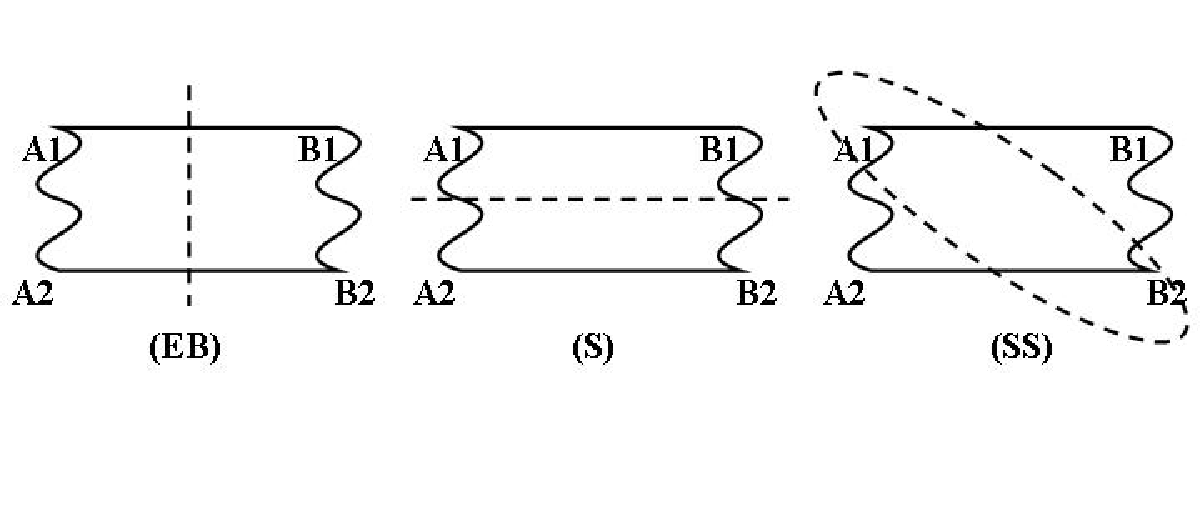
(a) an operation is separable iff the Jamiolkowski state is separable across the (A1A2)-(B1B2) split.
(b) an operation is equivalent to the swap operation, preceded by and followed by separable operations, iff the Jamiolkowski state is separable across the (A1B2)- (A2B1) split.
(c) an operation is entanglement breaking iff the Jamiolkowski state is separable across the (A1B1)- (A2B2) split.
A set of operations is bi-entangling if every operation lies within the convex hull of these three classes (a),(b) and (c). An operation is hence bi-entangling iff the Jamiolkowski state that represents it can be written as:
| (2) |
where is a probability distribution, the sets , , are also individual probability distributions, and all ’s on the r.h.s. are valid density matrices.
This is a convenient point to discuss the relationship between B-machines and SP-machines. It is clear from the above definition that B-machines contain the convex hull of the separable operations with separable+swap operations. However, they do not contain all possible separability preserving operations. This becomes apparent from consideration of the following Jamiolkowski state:
| where: | (3) | ||||
As is a valid density matrix with the reduced state of parties A1-A2 maximally mixed, it corresponds to the Jamiolkowski state of a valid quantum operation. When viewed as a state of four parties, also has the property that a GHZ-type state can be distilled from it by LOCC operations - simply by measuring the particle B2 in the computational basis. However, as the Jamiolkowski states of bi-entangling operations contain only two-particle entanglement, this means that cannot represent a bi-entangling operation. However, manifestly represents an SP operation, because the output qubits B1-B2 are always left in a separable state. Therefore we can also conclude that the conjecture made in HN that that SP operations convex hullseparable ops, separable+swap, is indeed true foot. In the above definition of B-machines, we have included the ability to make separable operations, separable+swap operations, and EB operations. One might be tempted to expand this definition to include all SP operations as well. However, operations such as have the capacity to probabilistically generate many-particle entanglement when accompanied by EB channels such as Bell-measurements, and so in our definition of B-machines we are forced to include the smaller classes of separable and separable+swap operations, and not the larger class of SP operations.
We would now like to use the class of B-machines defined above to obtain bounds on the classical tolerance of important universal gate sets. Suppose for example that we have a universal quantum computer consisting of the CNOT gate and a sufficient set of single qubit operations. If we add some noise to the CNOT such that it is taken to a bi-entangling operation, then the whole set is taken to a B-machine, and can be efficiently classically simulated. Hence to bound the classical threshold of the CNOT in our device, we would like to calculate the minimal noise required to turn the CNOT into a bi-entangling operation. In general such calculations are very difficult.
It is at this point that we must discuss the form of the noise model that we consider. In the rest of this article we adopt the standard probabilistic noise model, where qubits are affected incoherently. In this model whenever we would like to perform an ideal quantum operation , instead due to noise we are forced to perform an operation that is related to as follows:
| (4) |
where is a probability, and is some other quantum operation that represents the error. In this equation is measure of the error rate. Note that this is not the most general model of error, and not necessarily the most physical model either. Consider the example where our ideal operation is to simply preserve the state of a qubit, but in fact it undergoes a spontaneous emission at a sufficiently slow rate. This form of error cannot be written in the form of equation (4) unless the error parameter is set to (see e.g. NC, page 442). For more generic errors one would have to adopt some suitable metric on the set of quantum operations and use as a measure of error rate (see e.g. GLN for some possible metrics). Although several authors have considered more general models of error in relation to fault tolerance noise, the only prior work on classical tolerance has been within the framework of equation (4), and this is the model that we will follow here. In the case of Markovian, identical, and independent noise it should be possible to extend many of the techniques presented here to metric based noise quantification, although we will not pursue that avenue here. Within the probabilistic model, one can also make further restrictions, and constrain the form of to interesting forms of noise such as depolarization or dephasing. As with HN, however, our analysis will initially take to be a general quantum operation.
Given that our error model is probabilistic, our task is to find the minimal value such that there is a valid taking our ideal gate into the set of bi-entangling operations. In general this is likely to be a difficult task. However, for the case of the CNOT a great deal of symmetry is present that enables the calculation to be performed exactly. In order to see how this proceeds, it will be first helpful to consider the case that the two qubit gate is a general unitary , and examine some of the symmetry possessed by the Jamiolkowski state that represents .
For any 2-qubit unitary we have the trivial identity:
| (5) |
where are the standard Pauli operators. This identity, together with the fact that for any linear operator , can be used to show that the Jamiolkowski state representing commutes with all operators of the form:
| (6) |
It is not hard to verify that as we vary over the operators in equation (6) form a group (up to an unimportant phase), and moreover from the commutation relationships of the Pauli operators it follows that the group is abelian. It hence follows from Schur’s lemma that any operator that commutes with all operators of the form (6) is diagonal in the eigenbasis formed by the one-dimensional irreducible representations of the group (6). We can construct these irreducible representations quite easily. In fact, the group (6) is isomorphic to the group consisting of elements
| (7) |
as it is related to (6) by the unitary transformation . Hence we can utilize the stabilizer formalism for the Pauli group, and write the 16 common eigenstates of the operators in (6) as:
| (8) | |||||
where is a 4-bit string given by its components . It turns out that each of these eigen-projectors is a Jamiolkowski state for a valid quantum operation - the normalization and positivity are automatic, and the reduced density matrices over particles A1,A2 are all maximally mixed (this is in turn because is an irreducible representation). The Jamiolkowski state representing is in fact given by the projector corresponding to :
| (9) |
If we denote the Jamiolkowski state that represents by , then our task is to find the minimal probability such that for some quantum noise :
| (10) |
is the Jamiolkowski state of a bi-entangling operation. Now the properties of the CNOT allow us to make further simplifications. The CNOT is a member of the Clifford group, meaning that for any two Pauli operators we have that
| (11) |
where are other Pauli operators, and the symbol means that the two sides of the equation are equal up to an unimportant global phase. This means that the group (6) corresponding to the CNOT is actually a local group, where each element is a tensor product of Pauli operators acting on individual qubits of the Jamiolkowski state. We can therefore average (‘twirl’) over the group (6) any valid solution (10) corresponding to the CNOT, and as each is local, the bi-entangling properties of the equation will not be changed. This means that without loss of generality, for the CNOT we need only consider ‘twirled’ noise states that are also invariant under the action of the group. This means that we can set
| (12) |
where is a probability distribution of eigenvalues. If we have not constrained further the form of , then the form of the probability distribution can be left free. However, if we are restricting to be of a specific form such as depolarization or dephasing, then we will have to restrict the distribution accordingly. Our task is hence to find the minimal probability such that there exists a probability distribution (consistent with any further constraints upon the noise) such that the state:
| (13) |
is bi-entangling. Let us denote this optimal value of by . We can now try to perform this optimization for various possible constraints upon the noise:
(a) No constraints: In this case we need only restrict the s to be a probability distribution, and do not need to further constrain them. Take to be the maximal possible over all bi-entangling states invariant under the symmetry group (6). Then we clearly have that:
| (14) |
and hence as we have that:
| (15) |
This lower bound can be attained as we are free to choose the form of the noise as we wish. Hence , and our task is now to calculate . This is now an easier problem, as the fact that the set of bi-entangling states is the convex hull of separable, separable+swap, and EB states means that:
| (16) |
where are the maximal possible ’s over separable states, separable+swap states, and EB states respectively. This means that to work out the minimal generic noise required to turn the CNOT into a bi-entangling gate, we simply need to separately calculate the minimal noise required to take the CNOT into the different classes of separable, separable+swap, and EB, and take the lowest value. As each of these classes separately corresponds to separability across a particular partition of the parties in the Jamiolkowski state, we can apply the techniques developed in HN. Although we omit the details, it turns out that the Jamiolkowksi state representing the CNOT has only 1 ebit of maximal entanglement across the (A1B1)-(A2B2) splitting or the (A1B2)-(A2B1) splitting, but as with any two-qubit unitary has a full 2 ebits of maximal entanglement across the (A1A2)-(B1B2) splitting. Hence the CNOT is less robust to noise across the separable/separable+swap splittings. Furthermore, the results of vidal; HN show that the minimal noise that breaks the entanglement of the CNOT across the relevant splitting can always be chosen to be separable across that splitting. The result of all these observations is that the bounds derived in HN for generic noise are also optimal when considering B-machines as the classically tractable set. It is also interesting to note that if we do not ask for the noise to take us into the bi-entangling set, but instead ask to be taken into the entanglement breaking channels, then the above approach yields solutions for all unitary gates, not just the CNOT foot2.
(b) Separable noise, Separable+swap noise, Noise that is a mixture of Separable & Separable+swap: The previous paragraph points out that by the arguments of vidal; HN, the minimal generic noise that turns the CNOT into a bi-entangling gate can always be taken to be separable, or separable+swap. Hence the bounds derived in HN are also optimal w.r.t. these forms of noise, and where the classically tractable set is the set of B-machines.
(c) Depolarizing noise: The case of depolarizing noise on individual qubits is a little more tricky to handle than two particle noise. This is primarily because the depolarization is assumed to act independently upon the two qubits in the quantum gate. If we adopt the model in equation (56) of HN, with an error parameter the noisy operation is in fact:
| (17) |
where represents the single qubit depolarizing quantum operation,
| (18) |
and represents the ideal unitary quantum operation (we often represent a unitary and the corresponding quantum operation by the same letter - the meaning should be clear from the context). In particular we will take to be the CNOT operation. In order to derive un upper bound on the minimum value of required to make this noisy operation bi-entangling, we will first show that the (unnormalised) quantum operation corresponding to the central terms of equation (17):
| (19) |
is in fact a separable operation (not just SP) for any value of . Hence if the (unnormalised) operation corresponding to the outer terms:
| (20) |
is entanglement breaking, then the whole operation (17) is bi-entangling. First we must show that the central terms (19) correspond to a separable operation. Consider the operation , where is the CNOT. After a little algebraic manipulation of the Jamiolkowski state corresponding to the CNOT, it can be shown that the Jamiolkowski state of is:
Writing this out in the computational basis where represents the +1 eigenstate of the operator, and represents the -1 eigenstate of the operator, we find that may be written as an equal mixture of the following four pure states:
As each of these pure states is separable across the (A1B1)-(A2B2) split, it is clear that is a separable operation. Similarly, one can show that the Jamiolkowski state representing the operation is related to the state representing in the following way:
| (21) |
where the is a Hadamard rotation on each qubit, and SWAP1↔2 is the operation that interchanges A1 with A2 and B1 with B2. As is related to by local rotations followed by interchanging the labels , it is also separable across the (A1B1)-(A2B2) split, and hence both central terms in equation (17) correspond to separable operations.
It now remains for us to determine values of for which the outer terms (20) represent an entanglement breaking operation. The CNOT, as with any unitary on two-qubits, is represented by a Jamiolkowski state that is maximally entangled across the (A1B1)-(A2B2) splitting. The depolarizing operation on both qubits , on the other hand, is represented by a maximally mixed state. Hence if we are only considering the (A1B1)-(A2B2) splitting, the state representing the operation of equation (20) is essentially a maximally entangled state of two 4-level systems, mixed with a maximally mixed state. The conditions for such a state to be separable across the (A1B1)-(A2B2) splitting, and hence entanglement breaking, are well known, and correspond to:
| (22) |
giving that (20) is entanglement breaking whenever:
| (23) |
This means that the noisy CNOT gate is definitely bi-entangling whenever the depolarizing noise rate is greater than 67%. This is an improvement over the 74% bound derived in HN for exactly the same noise model, and hence shows that consideration of B-machines may lead to tighter bounds than consideration of separable machines alone. Of course the calculation here is not a full optimization over all bi-entangling gates - we have only calculated the minimal required to make the inner terms separable, and the outer terms entanglement breaking. This hence only provides an upper bound to the minimal required to make the CNOT bi-entangling, and hence there is a possibility that this calculation may be improved. However, as such full optimization is likely to be difficult, we leave it to another occasion.
It is also worth noting that the classical tolerance bound of 67% derived here applies to any two-qubit unitary for which the operations and are separable.
IV Bounds from the Gottesman-Knill theorem
In order to apply the Gottesman-Knill theorem GK to calculate bounds on the classical tolerance of quantum gates, we need to compute the minimal amounts of noise required to take all the gates in a particular machine into the Clifford class. Unfortunately this restricts severely the possible situations in which this approach may be applied. In previous examples we have calculated the classical tolerance of certain two-qubit gates with only very loose constraints on the other gates available to the machine. In this section we will calculate the classical tolerance of single qubit gates, assuming that the other gates in the machine are Clifford operations, where we define Clifford operations as follows:
Definition: Clifford operations. Those operations that can be performed by probabilistic application of Clifford group unitaries C, (ancilla) state preparation, and measurement in the computational basis.
We will ask how much noise is required to turn non-Clifford single qubit gates into a Clifford operation. The resulting bounds on the classical tolerance can be relatively low. For general single qubit operations we will show that the classical tolerance to generic noise is no greater than 75%, although on a case-by-case basis this can be made much stronger. For example for the gate, we find that 15% noise is minimal amount required to turn the gate into a Clifford operation.
In order to perform these calculations, at first it seems necessary to understand which single qubit operations can be implemented using Clifford group unitaries and ancillas prepared in the computational basis. However, we will not characterize this set exactly here, as to obtain optimal bounds for many interesting cases it turns out that it is sufficient to consider the effect that Clifford operations have upon a particular subset of single qubit states.
We will consider the set of states that is given by the convex hull of the Pauli operator eigenstates. This set is an octahedron that is shown in figure (2). Our choice of this set is inspired by the recent work of Bravyi & Kitaev BK, who consider which single qubit state supplies may allow the Clifford operations to become universal. We will first argue that the octahedron can only be mapped to within itself by Clifford operations, and use this fact to simplify the optimizations that we wish to perform.

Observation 0: The octahedron is closed under the action of Clifford operations.
Proof: Let us consider a system that is prepared in one of , where refers to the up/down eigenstates of the corresponding Pauli operator . These states correspond to the vertices of the octahedron . Suppose also that there are ancillae prepared in the computational basis, as can be prepared by Clifford operations. We need to calculate what possible final states of the system are possible given Clifford group unitary evolution of the system+ancilla & Clifford group measurements. As the entire input state is a stabilizer state GK; NC, the final state of system+ancilla will also be a stabilizer state that is uniquely specified by its stabilizer generators
where each is a product of Pauli operators. Hence from the standard theory of stabilizers, the final state of system+ancilla will be given by:
This equation may be expanded, and each element of the group that is generated by the stabilizer will contribute exactly one term in this expansion (this follows from the independence of the stabilizer generators NC). As any non-trivial Pauli operator is traceless, tracing out the ancilla qubits from each term will only lead to a contribution to the final reduced state of the system if the term is of the form , where , in which case the term will contribute to the system density matrix. Our goal is hence to find every group element of the form in the stabilizer group. As the identity is an element in each stabilizer group, we will at least have a contribution of (which is of course a requirement in the Bloch expansion of any single qubit state). However, we need to find all other terms of the form .
This task can be constrained as follows. Firstly, in each
stabilizer group each element is its own inverse. This means that
any non-trivial terms of the required form must actually be one of
the 6 possibilities or . Moreover, at
most only one of these 6 possibilities is present in each
stabilizer group, as if two or more are present, then repeated
multiplication we would force to be a member of the
stabilizer group (e.g. ), and this is not possible.
This means that input system states taken from the vertices of the
octahedron will be taken either to the maximally mixed state
, or one of the eigenstates of the operators
(corresponding to etc.). This
means that the vertices will be taken either to the maximally
mixed state, or to another vertex. Then by convexity the
octahedron can only be mapped onto or within itself by
Clifford operations.
This observation may be used to give lower bounds on the amount of noise required to take any particular unitary operation into a Clifford operation. Then by explicit construction we will be able to show that whenever the unitary is diagonal in the computational basis, that these lower bounds may be achieved, and are hence tight. First let us see why the above arguments allow us to construct lower bounds on the minimal noise level required. Consider a unitary gate of the form:
| (24) |
This gate acts upon the state to give:
| (25) |
We may visualize this by looking at the cross-section of the Bloch sphere given by the x-y plane. This is shown in figure (3), with the point representing corresponding to the action of the gate. One can see intuitively from the figure, and this can easily be shown rigorously, that the minimal noise level required to take the state into the octahedron is given by the ratio AB/AC from the figure.
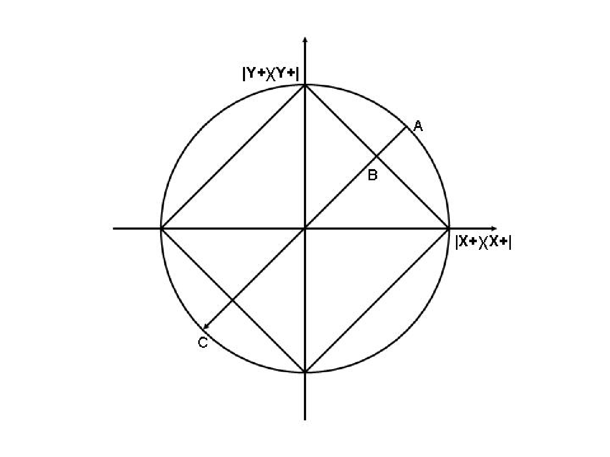
In the case of the gate, the ratio AB/AC corresponds to a noise level of:
| (26) |
If a noise level less than this amount could be added to the gate to turn it into a Clifford operation, then this would mean that the state would be mapped to outside the octahedron by the noisy operation. As this is not possible, we can assert that (26) is a lower bound on the amount of noise required to take the operation into the Clifford operations.
The utility of pictures such as figure (3) is that they may be used to show that bounds such as (26) are in fact also upper bounds, and are hence tight. The argument for this is strongly related to the construction presented BK for the programming of unitary operations in quantum states. Every state on the circumference of the Bloch sphere in the x-y plane corresponds to a pure state of the form:
| (27) |
These states are clearly isomorphic to the Jamiolkowski states representing each , simply by changing and :
| (28) |
Hence by using convexity every state in the x-y cross section of the Bloch sphere represents a valid quantum operation. From this isomorphism we see hence that each of the vertices represents a Clifford unitary: represents the identity gate , represents the Pauli Z rotation, state represents the so called phase gate NC, denoted by the letter :
and represents its inverse, . This mapping hence shows that bounds such as (26) can indeed be attained, as the x-y plane of the Bloch sphere maps directly into a problem concerning quantum operations and a subset of the Clifford operations. Hence for gates of the form we have the following statement:
Lemma 1: The minimal noise required to turn into a Clifford operation is equivalent to the minimal noise required to take the state into the octahedron in figure (3).
As shown above, in the case of the gate this lemma returns a minimal noise level is approximately 15%. The same procedure also yields sharp bounds for any unitary gate that may be diagonalised by Clifford group unitaries, as well as for any quantum operation that is a convex mixture of such unitaries.
We may also apply the above arguments to some cases where the noise is constrained to be of a specific form. Suppose for example that we wish to know how much dephasing noise is required to take the gate into the set of Clifford operations. The dephasing operation takes to the maximally mixed state, at the centre of the Bloch sphere in figure (3). On the other hand, when figure (3) is viewed as representing Jamiolkowski states of quantum operations, the centre of the circle in figure (3) also represents the dephasing operation. Hence the above arguments also show that:
Lemma 2: The minimal dephasing noise required to take any gate into a Clifford operation is identical to the minimal amount of maximally mixed state required to take the corresponding state into the octahedron in figure (3).
In the case of the gate this shows that approximately 30% dephasing noise is required to take the gate into the Clifford operations, or more precisely twice the value in equation (26):
| (32) |
Although the bounds on the classical noise threshold obtained in this way are quite low compared to bounds obtained in references AB; HN; R, the above procedure has the disadvantage that it applies only to very specific gate sets, whereas previous works have applied to much wider classes of machine. At the expense of increasing the bound, we can however, make the approach more general. For instance, we can show that the universal gate set consisting of Clifford operations augmented by any trace-preserving single qubit operation have a classical noise tolerance of no greater than 75 % on the additional single qubit operation. The argument proceeds as follows. Given any single-qubit trace preserving operation , we can always turn it into an operation that is a convex mixture of Clifford group operations by the following method. Instead of performing on an input state , we perform:
| (33) |
In the Jamiolkowski representation this quantum operation can be represented as:
This corresponds to a ‘Bell twirling’, and the resultant quantum operation is represented by a Bell diagonal state, which is a mixture of the four Pauli transformations. Hence by adding 75 % noise, any trace preserving single qubit operations may be taken to a probabilistic mixture of Clifford group operations, and so any machine consisting of {CNOT+single qubit gates} has a classical noise tolerance of at most 75 % on the single qubit gates.
V interpretation of the bounds.
The bounds derived in the previous sections give upper bounds to the fault tolerance of specific gates. For example, in the case of the gate set Clifford unitariesgate, they show that no fault-tolerant encoding can be found that protects against 15% general single gate noise. However, this does not mean that specific forms of noise cannot be tolerated to greater than 15%, but one must construct protection methods that specifically target that form of noise.
Furthermore, in the case of the approach based upon the Clifford group, our results show that if the Clifford gates in a gate set are noiseless, then the noise corresponding to lemma 1 may not be tolerated on an additional non-Clifford gate . However, it is possible that by mixing noise in with the Clifford gates as well, and not imposing that they be noiseless, one can recover the power to do universal quantum computation. Indeed, we have been able to construct examples where mixing a certain type of noise to the gate from a universal set Clifford unitaries, leads to classically tractable evolution, but mixing the same noise same with the Clifford gates as well as restores the ability to perform universal quantum computation. Although we do not include the details here, the examples that we have are all quite extreme, and work because noise that turns the non-Clifford gate into a Clifford operation can also take the Clifford unitaries out of the Clifford group dep. Nevertheless, in these examples the fault tolerant encoding methods that restore universality are very specific, and cannot be used to tackle general noise of the same level.
VI Conclusions
We have presented a class of operations - the bi-entangling operations - that may be efficiently simulated classically, as they are only capable of generating two party entanglement. In some situations this class of operations may give tighter bounds than currently known on the classical noise tolerance of quantum gates. One example is the case of depolarizing noise on the CNOT, for which we show that 67% noise is sufficient to make the subsequent evolution efficiently tractable classically, compared to the best previous bound of 74%. Another extreme case is with measurement based computation, where we observe that two-qubit non-degenerate measurements cannot enable exponential speedup over classical computation. It may be difficult to extend the class of bi-entangling operations and still generate a class that is efficiently tractable. This is because any natural generalizations to higher numbers of input particles enable perfect quantum computation, and any extensions that still involve two-particle gates are hampered by the subtle interplay between separability preserving and separable gates.
In the second half of this work we turn to bounds on classical tolerance that may be derived from the Gottesman-Knill theorem. The subsequent bounds (e.g. 30% depolarizing noise on the gate, 15% for general single-gate noise) can be relatively low for this kind of approach.
In general it is quite likely that the bounds derived here may be improved. One interesting possibility is that a hybrid of the approaches used by AB and HN may be used to understand when slightly non-separable gates may be efficiently simulated classically, albeit with a noise model more in the spirit of AB; R, where noise is applied to every qubit at every time step.
In terms of the Clifford gate based work, it seems quite possible that if the recent conjecture of Bravyi & Kitaev BK is true, then the fault tolerant threshold gates of the form can indeed be made fault tolerant to the noise levels derived here (and implied by their work). Their conjecture implies that a supply of single qubit quantum states from outside the octahedron may be ‘purified’ to certain ‘magic’ pure states by the use of Clifford operations only. As Clifford operations may be made fault tolerant to some degree via encoding schemes based on Clifford operations only (see e.g. NC and references therein), it may be possible that the 15% noise level on the gate may indeed be tolerated as long as the remaining Clifford operations act within their own (potentially much tighter) fault tolerant threshold.
These results show the potential of analyzing classical tractability with the aim of bounding from above fault tolerance thresholds. Moreover, investigating the quantum/classical computational transition for (noisy) quantum evolution is important in its own right AB; BK, particularly as there is the possibility of ‘intermediate’ quantum computation. It may well be the case that noisy quantum devices cannot be simulated efficiently classically, yet cannot be used for fault tolerant quantum computation. This would imply the existence of an intermediate physical device - such as a noisy quantum system controlled by a universal classical computer - which is clearly universal for computation, is better-than-classical as it can simulate itself efficiently, and yet is not as powerful as a full quantum computer. Such intermediate devices may be easier to construct, and hence may provide a more achievable experimental target.
VII Acknowledgements
We thank Koenraad Audenaert and Terry Rudolph for interesting discussions. We acknowledge financial support by US-Army through grant DAAD 19-02-0161, The Nuffield Foundation, a Royal Society Leverhulme Trust Senior Research Fellowship and the EU Thematic Network QUPRODIS.
References
- (1) R. Jozsa and N. Linden, (quant-ph/0201143); G. Vidal, Phys. Rev. Lett. 91, 147902 (2003) (quant-ph/0301063).
- (2) D. Aharonov and M. Ben-Or, FOCS 1996 (quant-ph/9611029); D. Aharonov, M. Ben-Or, R. Impagliazzo and N. Nisan (quant-ph/9611028). see also D. Aharonov, Phys. Rev. A. 62, 062311 (2000) (quant-ph/9910081) for related work.
- (3) A. Harrow and M. Nielsen, Phys. Rev. A 68, 012308 (2003) (quant-ph/0301108).
- (4) L. Valiant, SIAM J. Comput. 31, 4, pp. 1229 (see also Proc. ACM STOC, pp. 114-123, 2001 for preliminary version); B. M. Terhal and D. P. Divincenzo, Phys. Rev. A. 65, 032325 (2002) (quant-ph/0108010); E. Knill, (quant-ph/0108033); S. Bravyi, (quant-ph/0404180).
- (5) A. Razborov, (quant-ph/0310136).
- (6) S. Bravyi and A. Kitaev, (quant-ph/0403025).
- (7) Stated in thesis of D. Gottesman Stabilizer Codes and Quantum Error Correction, California Institute of Technology, 1997. For recent improvements see also S. Aaronson & D. Gottesman, (quant-ph/0406196).
- (8) Definitions of all gates in this paper, as well as a good review of the stabilizer formalism, may be found in the textbook ‘Quantum Information & Quantum Computation’, M. Nielsen & I. Chuang, Cambridge, (2001).
- (9) A. Jamiolkowski, Rep. Math. Phys. 3, 275 (1972).
- (10) E.M. Rains, Phys. Rev. A 60, 173 (1999) (quant-ph/9809078); E.M. Rains, Phys. Rev. A 60, 179 (1999) (quant-ph/9809082).
- (11) J.I. Cirac, W. Dür, B. Kraus and M. Lewenstein, Phys. Rev. Lett. 86, 544 (2001) (quant-ph/0007057).
- (12) A.S. Holevo, Russian Math. Surveys 53, 1295-1331 (1999) (quant-ph/9809023).
- (13) see e.g. R. Raussendorf, D. E. Browne, and H. J. Briegel, Phys. Rev. A 68, 022312 (2003) (quant-ph/0108118); M. Nielsen, Phys. Lett. A, 308, 96 (2003) (quant-ph/0108020); S. A. Fenner and Y. Zhang, (quant-ph/0111077); S. Perdrix and P. Jorrand, (quant-ph/0404146)
- (14) D. W. Leung, Int. J. Quant. Inf., 2, 33 (2004) (quant-ph/0111077).
- (15) D. Gottesman and I. Chuang, Nature 402, 390 (1999), (quant-ph/9908010).
- (16) The Clifford group is the set of unitaries that by conjugation map tensor products of Pauli of operators to tensor products of Pauli operators, i.e. we always have , where the are Pauli operators.
- (17) For example, it can be shown that the W-class of entangled pure states cannot be created by Clifford operations from computational basis inputs. The W class represents an important form of three party entanglement, as defined by W. Dür, G. Vidal, and J. I. Cirac, Phys. Rev. A 62, 062314 (2000)).
- (18) A. Gilchrist, N. K. Langford and M. A. Nielsen, (quant-ph/0408063).
- (19) In fact the quantum operation conjectured by HN as an example of an SP operation that is not in the convex hull of separable and separable+swap operations is in fact correct. The proof works by noting that LOCC operations on separable and separable+swap Jamiolkowski states cannot result in entanglement between particles A1,A2. However, the SP operation presented in HN has this property.
- (20) D. Aharanov and M. Ben-Or, (quant-ph/9906129). B. M. Terhal and G. Burkard, (quant-ph/0402104); R. Alicki, M. Horodecki, P. Horodecki, and R. Horodecki. Phys. Rev. A, 65 062101, (2002) (quant-ph/0105115); M. Nielsen and C. M. Dawson, (quant-ph/0405134).
- (21) The symmetry group (6) is local across the (A1A2)-(B1B2) split for all unitaries, and so group averaging does not change the EB properties of any EB state. Hence in looking for the minimal noise that takes a given unitary into an EB operation, the form of the noise may be restricted to being symmetric. As any state that is averaged under (6) is automatically a valid Jamiolkowski state, may immediately utilise the results on robustness of entanglement for density matrices, and we find that all unitaries are equally robust to being taken to an EB channel by generic noise - this is unsurprising as all unitaries have Jamiolkowski states that are maximally entangled across the EB split. We find that a minimum of 3/4 = 75% noise is required to take a two-qubit unitary into an entanglement breaking channel.
- (22) G. Vidal and R. Tarrach, Phys. Rev. A. 59 141-155 (1999) (quant-ph/9806094).
- (23) The term ‘same noise’ does not have a strong meaning here, as whether one form of noise on one gate is the ‘same’ as a form of noise on another gate strongly depends upon precise physics of real devices. For example, the same physical source of noise, such as a fluctuating magnetic field, may affect different gates in very different ways.
- (24) Of course to do this the noise itself must not be a Clifford operation, so for example dephasing cannot display this phenomenon.