Optimized quantum implementation of elliptic curve arithmetic over binary fields

Phillip Kaye Thanks: prkaye@iqc.ca, School of Computer Science, University of Waterloo, Waterloo, ON, Canada. Christof Zalka Thanks: zalka@iqc.ca, Department of Physics, University of Waterloo.

Abstract

Shor’s quantum algorithm for discrete logarithms applied to elliptic curve groups forms the basis of a “quantum attack” of elliptic curve cryptosystems. To implement this algorithm on a quantum computer requires the efficient implementation of the elliptic curve group operation. Such an implementation requires we be able to compute inverses in the underlying field. In [PZ03], Proos and Zalka show how to implement the extended Euclidean algorithm to compute inverses in the prime field $\textnormal{GF}(p)$ . They employ a number of optimizations to achieve a running time of $O(n^{2})$ , and a space-requirement of $O(n)$ qubits (there are some trade-offs that they make, sacrificing a few extra qubits to reduce running-time). In practice, elliptic curve cryptosystems often use curves over the binary field $\textnormal{GF}(2^{m})$ . In this paper, we show how to implement the extended Euclidean algorithm for polynomials to compute inverses in $\textnormal{GF}(2^{m})$ . Working under the assumption that qubits will be an ‘expensive’ resource in realistic implementations, we optimize specifically to reduce the qubit space requirement, while keeping the running-time polynomial. Our implementation here differs from that in [PZ03] for $\textnormal{GF}(p)$ , and we are able to take advantage of some properties of the binary field $\textnormal{GF}(2^{m})$ . We also optimize the overall qubit space requirement for computing the group operation for elliptic curves over $\textnormal{GF}(2^{m})$ by decomposing the group operation to make it “piecewise reversible” (similar to what is done in [PZ03] for curves over $\textnormal{GF}(p)$ ).

1 Introduction

A very significant potential application of quantum computers lies in their ability to efficiently solve the problem of finding discrete logarithms over finite groups. It is this ability that makes quantum computers capable, in principle, of undermining the security of elliptic curve cryptographic systems, which are widely used by industry and government to protect sensitive information. There is no known classical algorithm for solving the discrete logarithm problem in polynomial time. In 1994, Peter Shor [Sho94] described a quantum algorithm for solving this problem in polynomial time.

The construction of medium- or large-scale quantum computers has turned out to be an enormous technological challenge. For most of the proposed (practical) schemes for implementing quantum computers, qubits are a very ‘expensive’ resource. Thus there is a significant practical interest in optimizing quantum algorithms to use as few qubits as possible. In [PZ03], Proos and Zalka give an optimized implementation of the discrete logarithm algorithm, for the particular case of elliptic curve groups. They consider only elliptic curves over the prime fields $\textnormal{GF}(p)$ . Many elliptic curve cryptosystems use elliptic curves over the binary fields $\textnormal{GF}(2^{m})$ however. So it is important to examine the number of qubits required to implement the discrete logarithm algorithm for elliptic curve groups over these binary fields. In this direction, we show how to decompose the group operation into a series of smaller, individually reversible, steps (following the approach taken in [PZ03]). Some of these steps will involve divisions of elements in the binary field $\textnormal{GF}(2^{m})$ . To solve this problem, we show how to implement the extended Euclidean algorithm for polynomials, and optimize this implementation to use few qubits.

2 Elliptic curves over $\textnormal{GF}(2^{m})$

An elliptic curve over a field $F$ is the set of points $(x,y)\in F^{2}$ satisfying

y^{2}+a_{1}xy+a_{3}y=x^{3}+a_{2}x^{2}+a_{4}x+a_{5},

subject to some additional conditions on the constants $a_{1},\ldots,a_{5}\in F$ , together with a ‘point at infinity’, denoted $\mathcal{O}$ . For the particular case of curves over the finite fields $\textnormal{GF}(2^{m})$ , the defining equation and additional conditions simplify as follows.

Case 1:

$a_{1}\neq 0$ (non-supersingular curves)

$y^{2}+xy=x^{3}+ax^{2}+b\hskip 14.22636pt,\hskip 14.22636ptb\neq 0.$
Case 2:

$a_{1}=0$ (supersingular curves)

$y^{2}+cy=x^{3}+ax+b\hskip 14.22636pt,\hskip 14.22636ptc\neq 0.$

An elliptic curve over $\textnormal{GF}(2^{m})$ is the set of points $(x,y)\in\textnormal{GF}(2^{m})\times\textnormal{GF}(2^{m})$ that satisfy one of the above two formulae, together with the point at infinity $\mathcal{O}$ . A particular curve of one of the above types is specified by giving values to the constants $a,b$ (and $c$ in the case of a supersingular curve). The set of points on a given elliptic curve forms a group under the following operation of addition. Let $P=(x_{1},y_{1})$ and $R=(x_{2},y_{2})$ , where $P\neq R$ , be two distinct points on a curve over $\textnormal{GF}(2^{m})$ . The point $P+R$ is defined as follows.

Case 1:

non-supersingular curves

P+R=\begin{cases}\mathcal{O}\hskip 14.22636pt\text{if }(x_{2},y_{2})=(x_{1},x_{1}-y_{1})\\ (x_{3},y_{3})\hskip 14.22636pt\text{otherwise, }\end{cases}

\text{where}\hskip 14.22636ptx_{3}=\lambda^{2}+\lambda+x_{1}+x_{2}+a\hskip 14.22636pt,\hskip 14.22636pty_{3}=\lambda(x_{1}+x_{3})+x_{3}+y_{1}

\lambda=\frac{y_{1}+y_{2}}{x_{1}+x_{2}}.

Case 2:

supersingular curves

P+R=\begin{cases}\mathcal{O}\hskip 14.22636pt\text{if }(x_{2},y_{2})=(x_{1},y_{1}+c)\\ (x_{3},y_{3})\hskip 14.22636pt\text{otherwise, }\end{cases}

\text{where}\hskip 14.22636ptx_{3}=\lambda^{2}+x_{1}+x_{2}\hskip 14.22636pt,\hskip 14.22636pty_{3}=\lambda(x_{1}+x_{3})+y_{1}+c

\lambda=\frac{y_{1}+y_{2}}{x_{1}+x_{2}}.

Following the argument in [PZ03], we can avoid dealing with the cases $P=R$ (point doubling) $P=-R$ , and $R=\mathcal{O}$ , and restrict ourselves to the generic group addition formulae in terms of $x_{3},y_{3}$ above. The key observation is that in a superposition (such as we would have in the quantum discrete logarithm algorithm), situations other than the generic case will occur for only a small fraction of the elements in superposition, and so by ignoring them the fidelity loss will be negligible.

3 The discrete logarithm algorithm for elliptic curve groups

Let $G$ be a cyclic group, and let $\alpha$ be a generator for $G$ . The discrete logarithm problem with respect to the base $\alpha$ is the following. Given a group element $\beta\in G$ , find the unique integer $d\in[0,|G|-1]$ such that $\beta=\alpha^{d}$ . Recall that Shor’s quantum algorithm for solving the discrete logarithm problem makes use of a unitary operator that performs

|x\rangle|y\rangle|z\rangle\rightarrow|x\rangle|y\rangle|z\oplus\alpha^{x}\beta^{y}\rangle,\hskip 28.45274pt(\ast)

where $x$ and $y$ are integers in the range $[0,\ldots,|G|-1]$ .

Consider an elliptic curve $E$ and let $P$ be a point on $E$ . Consider the cyclic subgroup of the elliptic curve group generated by $P$ . We are interested in solving the discrete logarithm problem for this subgroup. The group operation is written additively, so the discrete logarithm problem is the following. Given a point $Q$ in the subgroup generated by $P$ , find the unique integer $d\in[0,\ldots,\text{order}(P)-1]$ such that $Q=dP$ . The unitary operation $(\ast)$ used in Shor’s algorithm performs

|x\rangle|y\rangle|z\rangle\rightarrow|x\rangle|y\rangle|z\oplus(xP+yQ)\rangle.

Employing the semiclassical Fourier transform of Griffiths and Niu [GN95] as detailed in [PZ03], for the discrete logarithm algorithm it suffices to be able to implement

|S\rangle\rightarrow|S+A\rangle\hskip 14.22636ptS,A\in E\text{ and }A\text{ is fixed and `classically known'}.

Writing $S=(x,y)$ and $A=(\alpha,\beta)$ , we want to implement

|(x,y)\rangle\rightarrow|(x,y)+(\alpha,\beta)\rangle.

4 Decomposing the group operation

We now show how to decompose the group operation for curves over $\textnormal{GF}(2^{m})$ into a sequence of individually reversible steps. Doing so allows the implementation of the group operation with a smaller number of ancillary qubits.

We will use the following notation. When we write $x\rightarrow y$ , we are referring to a (not necessarily reversible) computation transforming the value $x$ into the value $y$ . When we write $x\hskip 5.69054pt\leftrightarrow\hskip 5.69054pty$ , we are referring to a reversible computation which can be seen as transforming $x$ into $y$ , or as transforming $y$ into $x$ .

For a fixed point $(\alpha,\beta)$ , define $(x^{\prime},y^{\prime}):=(x,y)+(\alpha,\beta)$ . We want to decompose the operation

|(x,y)\rangle\rightarrow|(x^{\prime},y^{\prime})\rangle.

For simplicity, in the following we will write the values without the Dirac ket symbols.

Case 1:

non-supersingular curves
We have

\lambda=\frac{y+\beta}{x+\alpha}=\frac{x^{\prime}+y^{\prime}}{x^{\prime}+\alpha}.

The group operation is decomposed as

	$\displaystyle x,y$	$\displaystyle\hskip 5.69054pt\leftrightarrow\hskip 5.69054ptx+\alpha,y+\beta\hskip 5.69054pt\leftrightarrow\hskip 5.69054ptx+\alpha,\lambda=\frac{y+\beta}{x+\alpha}$
		$\displaystyle\hskip 5.69054pt\leftrightarrow\hskip 5.69054ptx^{\prime}+\alpha,\lambda=\frac{x^{\prime}+y^{\prime}}{x^{\prime}+\alpha}\hskip 5.69054pt\leftrightarrow\hskip 5.69054ptx^{\prime}+\alpha,x^{\prime}+y^{\prime}\hskip 5.69054pt\leftrightarrow\hskip 5.69054ptx^{\prime},x^{\prime}+y^{\prime}\hskip 5.69054pt\leftrightarrow\hskip 5.69054ptx^{\prime},y^{\prime}.$

The second step in the above decomposition is a division, and the fourth step is a multiplication, where in each case one of the operands is uncomputed in the process. All the other steps involve only additions (and the third step also requires the squaring of $\lambda$ ). It turns out that the number of qubits required to perform the group operation is bounded by the number of qubits required to perform a division or multiplication where one of the operands is uncomputed in the process.

Case 2:

supersingular curves
We have

\lambda=\frac{y+\beta}{x+\alpha}=\frac{y^{\prime}+c+\beta}{x^{\prime}+\alpha}.

The group operation is decomposed as

	$\displaystyle x,y$	$\displaystyle\hskip 5.69054pt\leftrightarrow\hskip 5.69054ptx+\alpha,y+\beta\hskip 5.69054pt\leftrightarrow\hskip 5.69054ptx+\alpha,\lambda=\frac{y+\beta}{x+\alpha}$
		$\displaystyle\hskip 5.69054pt\leftrightarrow\hskip 5.69054ptx^{\prime}+\alpha,\lambda=\frac{y^{\prime}+c+\beta}{x^{\prime}+\alpha}\hskip 5.69054pt\leftrightarrow\hskip 5.69054ptx^{\prime}+\alpha,y^{\prime}+c+\beta\hskip 5.69054pt\leftrightarrow\hskip 5.69054ptx^{\prime},y^{\prime}.$

As in the non-supersingular case, the second step in the above decomposition is a division, and the fourth step is a multiplication, where in each case one of the operands is uncomputed in the process. The other steps involve only additions, and one squaring. So again the qubit-space requirement for the group operation is that for a division or multiplication where one of the operands is uncomputed in the process.

In both the supersingular and non-supersingular case, the qubit space requirement of the group operation is determined by that of performing a division or multiplication, where one of the operands is uncomputed in the process. Such a multiplication can be achieved by running such a division backwards, so we turn our attention to implementing divisions of the form $x,y\hskip 5.69054pt\leftrightarrow\hskip 5.69054ptx,y/x$ , using as few qubits as possible. Following [PZ03] the division is decomposed into the following four reversible steps.

x,y\overset{E}{\hskip 5.69054pt\leftrightarrow\hskip 5.69054pt}1/x,y\overset{m}{\hskip 5.69054pt\leftrightarrow\hskip 5.69054pt}1/x,y,y/x\overset{E}{\hskip 5.69054pt\leftrightarrow\hskip 5.69054pt}x,y,y/x\overset{m}{\hskip 5.69054pt\leftrightarrow\hskip 5.69054pt}x,0,y/x.

The letters over the arrows are $m$ for standard polynomial multiplication, and $E$ for “Euclid’s algorithm”. The second $m$ is really a standard polynomial multiplication run backwards to uncompute $y$ . We know how to implement standard multiplication in $\textnormal{GF}(2^{m})$ using $2m$ qubits by [BBF03], so it remains to show how to implement the extended Euclidean algorithm for polynomials to compute inverses in $\textnormal{GF}(2^{m})$ .

5 The extended Euclidean algorithm for polynomials

Suppose $A(z)$ and $B(z)$ are two binary polynomials in the variable $z$ , of degrees less than $m$ (i.e. $A,B\in\textnormal{GF}(2^{m})$ ). Suppose $A$ and $B$ are not both 0, and are such that $\deg(A)\leq\deg(B)$ . The greatest common divisor of $A$ and $B$ , denoted $\gcd(A,B)$ , is the binary polynomial of highest degree that divides both $A$ and $B$ . The classical Euclidean algorithm for finding $\gcd(A,B)$ is based on the fact that $\gcd(A,B)=\gcd(B-CA,A)$ , for all binary polynomials $C$ . If we divide $B$ by $A$ (by standard long division of polynomials), obtaining a quotient polynomial $q(z)$ and a remainder polynomial $r(z)$ satisfying $B=qA+r$ , then $\deg(r)<\deg(A)$ . By the fact observed above, we have $\gcd(A,B)=\gcd(r,A)$ . The classical Euclidean algorithm for polynomials makes this replacement repeatedly until one of the arguments is 0. If we set $r_{0}=A$ and $r_{1}=B$ , the Euclidean algorithm performs the following sequence of divisions:

$\displaystyle r_{0}$	$\displaystyle=q_{1}r_{1}+r_{2},$	$\displaystyle\hskip-28.45274pt0<\deg(r_{2})<\deg(r_{1})$
$\displaystyle r_{1}$	$\displaystyle=q_{2}r_{2}+r_{3},$	$\displaystyle\hskip-28.45274pt0<\deg(r_{3})<\deg(r_{2})$
	$\displaystyle\hskip 5.69054pt\vdots$	$\displaystyle\hskip 5.69046pt\vdots$
$\displaystyle r_{m-2}$	$\displaystyle=q_{m-1}r_{m-1}+r_{m},$	$\displaystyle\hskip-28.45274pt0<\deg(r_{m})<\deg(r_{m-1})$
$\displaystyle r_{m-1}$	$\displaystyle=q_{m}r_{m}+0.$

The fact above gives us the corresponding sequence of equalities:

\gcd(r_{0},r_{1})=\gcd(r_{1},r_{2})=\ldots=\gcd(r_{m-1},r_{m})=\gcd(r_{m},0).

At this point we have the result, since $\gcd(r_{m},0)=r_{m}$ . The algorithm is guaranteed to terminate, since the degree of one of the arguments strictly decreases in each step. Moreover, the algorithm is efficient because the number of iterations is bounded by the degree of $A$ (which is at most $m$ ).

Recall that the $\gcd$ of two integers $a,b$ can always be written as a linear combination of $a$ and $b$ having integral coefficients. The same is true for the $\gcd$ of two polynomials $A,B$ . That is, there exist polynomials $k,k^{\prime}$ in $\textnormal{GF}(2^{m})$ such that

\gcd(A,B)=kA+k^{\prime}B.

The extended Euclidean algorithm for polynomials is the same as the Euclidean algorithm for polynomials except that it also keeps track of the ‘coefficient’ polynomials $k,k^{\prime}$ above. It does so through the following recurrences.

k_{j}=\begin{cases}1&\text{ if }j=0\\ 0&\text{ if }j=1\\ k_{j-2}-q_{j-1}k_{j-1}&\text{ if }j\geq 2\end{cases}

and

{k^{\prime}}_{j}=\begin{cases}0&\text{ if }j=0\\ 1&\text{ if }j=1\\ {k^{\prime}}_{j-2}-q_{j-1}{k^{\prime}}_{j-1}&\text{ if }j\geq 2.\end{cases}

It is not hard to show that for $0\leq j\leq m$ we have $r_{j}=k_{j}r_{0}+{k^{\prime}}_{j}r_{1}$ , where the $r_{j}$ ’s are defined as in the Euclidean algorithm for polynomials, and the $k_{j}$ and the ${k^{\prime}}_{j}$ are defined by the above recurrences.

For reference, we write the extended Euclidean algorithm for polynomials in pseudo-code below. The notation $x\leftarrow y$ is intended to mean that we assign the value of $y$ to the variable named $x$ .

EXTENDED EUCLIDEAN ALGORITHM FOR POLYNOMIALS

$A_{0}\leftarrow A$
$B_{0}\leftarrow B$
$k_{0}\leftarrow 1$
$k\leftarrow 0$
${k^{\prime}}_{0}\leftarrow 0$
$k^{\prime}\leftarrow 1$
$q\leftarrow\left\lfloor\frac{A_{0}}{B_{0}}\right\rfloor$
$r\leftarrow A_{0}-qB_{0}$
while $r>0$ do
1. temp $\leftarrow{k^{\prime}}_{0}-qk^{\prime}$
2. ${k^{\prime}}_{0}\leftarrow k^{\prime}$
3. $k^{\prime}\leftarrow$ temp
4. temp $\leftarrow k_{0}-qk$
5. $k_{0}\leftarrow k$
6. $k\leftarrow$ temp
7. $A_{0}\leftarrow B_{0}$
8. $B_{0}\leftarrow r$
9. $q\leftarrow\left\lfloor\frac{A_{0}}{B_{0}}\right\rfloor$
10. $r\leftarrow A_{0}-qB_{0}$
return $(r,k,k^{\prime})$

Inverses in $\textnormal{GF}(2^{m})$ can be computed using the extended Euclidean algorithm for polynomials, as follows. Suppose $f(z)$ is an irreducible polynomial of degree $m$ , and let $C(z)$ be a binary polynomial of degree $\leq m-1$ . Then $\gcd(C,f)=1$ , and the extended Euclidean algorithm for polynomials finds binary polynomials $k$ and $k^{\prime}$ such that $kC+k^{\prime}f=1$ . But this means that $kC\equiv 1(\text{mod }f)$ , and so $k\equiv C^{-1}(\text{mod }f)$ . The coefficient $k^{\prime}$ of $f$ is not needed for the inversion of $C$ , and so we only need to record the coefficient $k$ of $C$ throughout the algorithm.

6 Naive Implementation of the extended Euclidean algorithm for polynomials

We now turn our attention to quantum implementations of the extended Euclidean algorithm for polynomials for computing the inverse of an element $C$ . Following [PZ03], our implementations will maintain two ordered pairs $(a,A)$ and $(b,B)$ ., where $A$ and $B$ record the sequence of remainders in the Euclidean algorithm for polynomials, and $a$ and $b$ record the updated coefficient of $C$ for each of the past two iterations of the algorithm . We call these ordered pairs Euclidean pairs. The algorithm begins with $(a,A)=(1,C)$ , and $(b,B)=(0,f)$ (where $f$ is an irreducible polynomial of degree $m$ ). Note that $\deg(C)\leq m-1<m=\deg(f)$ . We will always store the Euclidean pair with the smaller-degree polynomial in the second co-ordinate first. That is, we store the Euclidean pairs in the order

(a,A)\hskip 2.84526pt,\hskip 2.84526pt(b,B)

where $\deg(A)<\deg(B)$ . We then want to perform long division of $B$ by $A$ , obtaining a quotient polynomial $q$ and a remainder polynomial $r$ satisfying $B=qA-r=qA+r$ (the second equality follows since the field is binary), where $q$ is the quotient polynomial of $B/A$ , which we denote as $q=\left\lfloor B/A\right\rfloor$ . We will then replace $B$ by $r=B+qA$ , and $b$ by $b+qa$ . Since $\deg(r)<\deg(A)$ , after the above replacement we will have to interchange the Euclidean pairs to maintain the ordering so that the pair with the smaller-degree polynomial in the second co-ordinate appears first. So one iteration of the algorithm can be written as

(a,A)\hskip 2.84526pt,\hskip 2.84526pt(b,B),0\longrightarrow(b+qa,B+qA)\hskip 2.84526pt,\hskip 2.84526pt(a,A)\hskip 2.84526pt,\hskip 2.84526ptq\hskip 28.45274pt\text{where }q=\left\lfloor B/A\right\rfloor.

At the beginning of the Euclidean algorithm, we start with $a=1,b=0,A=C,B=f$ , and so $\deg(A)<\deg(B)$ and $\deg(a)>\deg(b)$ . It is easy to see that this condition is preserved in every iteration of the algorithm. This implies that we will have $\left\lfloor\frac{b}{a}\right\rfloor=0$ . So we can write

q=\left\lfloor\frac{b+qa}{a}\right\rfloor.

So while $q$ is computed from the second co-ordinates of the Euclidean pairs $(a,A),(b,B)$ , it can be uncomputed from the first coordinates of the modified Euclidean pairs $(b+qa,B+qA),(a,A)$ . Thus each iteration of the Euclidean algorithm is individually reversible, and can be written as

(a,A)\hskip 2.84526pt,\hskip 2.84526pt(b,B)\hskip 5.69054pt\leftrightarrow\hskip 5.69054pt(b+qa,B+qA)\hskip 2.84526pt,\hskip 2.84526pt(a,A)\hskip 28.45274pt\text{where }q=\left\lfloor B/A\right\rfloor.

This is decomposed into the following three individually reversible steps:

	$\displaystyle A\hskip 2.84526pt,\hskip 2.84526ptB,0$	$\displaystyle\hskip 5.69054pt\leftrightarrow\hskip 5.69054ptA\hskip 2.84526pt,\hskip 2.84526ptB+qA\hskip 2.84526pt,\hskip 2.84526ptq$
	$\displaystyle a\hskip 2.84526pt,\hskip 2.84526ptb\hskip 2.84526pt,\hskip 2.84526ptq$	$\displaystyle\hskip 5.69054pt\leftrightarrow\hskip 5.69054pta+qb\hskip 2.84526pt,\hskip 2.84526ptb,0$
		SWAP

where “SWAP” refers to the operation of switching the two Euclidean pairs. Since $\deg(b)<\deg(a+qb)$ , the second operation above is simply the reverse of the first operation.

To perform the division $A,B,0\hskip 5.69054pt\leftrightarrow\hskip 5.69054ptA,B+qA,q$ we can use long division of the binary polynomial $B$ by $A$ . To implement this long division, the basic idea is to shift $A$ all the way to the left (i.e. we shift $A$ left by $m-\deg(A)-1$ bits). Then we start shifting $A$ to the right one bit at a time, each time conditionally doing a subtraction. For the binary field $\textnormal{GF}(2^{m})$ this is simplified by virtue of the fact that subtraction is the same as addition, and is achieved by a bitwise XOR operation. This bitwise XOR can be implemented quantumly using CNOT gates, and no ancillary qubits. (Furthermore, these CNOTs could in principle be performed in parallel, allowing us to do addition in a single step.) Note that in our long divisions we are doing more work than necessary. Often the degree of $B$ will be less than $m-1$ , and so it would not be necessary to shift $A$ all the way to the left (we could just shift it so the most significant bits of $A$ and $B$ line-up). For simplicity, in the naive implementation we do not take advantage of this fact, but will do so when we look at an optimized implementation.

6.1 Implementing some tools

To implement the long division, there are some subcomponents that we will need to implement. We describe implementations of some of these subcomponents here, optimizing for the number of qubits.

In what follows, we will show how to implement some operation, and then use that operation controlled on the value(s) of some other qubit(s). We need to consider whether this can be done without the requirement for any additional qubits, or an unreasonable increase in the running time. Fortunately, by [BBC+95], given a gate performing $U$ , we can construct a gate performing a controlled- $U$ (that is, $U$ conditioned on a control qubit being in state $|1\rangle$ ) with no additional ancillary qubits, and a small overhead in running time. Using this result repeatedly, we can implement $U$ conditioned on any desired pattern of control qubits (e.g. $U$ may be applied only when a three-qubits control register is in the state $|101\rangle$ ) with no additional ancillary qubits, and a small overhead in running time. We will use this result implicitly in the following.

For the long division, we will need to compute the degree of $A$ . The circuit shown in Figure 1 accomplishes this. Each of the hollow circles in the figure denotes a $0$ -control (that is, the $(-1)$ operation is applied if the control qubit is $|0\rangle$ ). To uncompute the degree, we can simply run the circuit shown in Figure 1 backwards.

Figure 1: Circuit to compute the degree of

A\in GF(2^{m})

The circuit in Figure 1 uses a sequence of $m$ decrementing (-1) gates, each of which is controlled by the values of some of the qubits of $|A\rangle$ . These decrementing gates update the value of $\deg(A)$ , being computed into a $\left\lceil\log(m-1)\right\rceil$ -qubit register. In Figure 2, we show how to implement an incrementing (+1) gate using only one additional ancillary qubit.

. . . . . . . . . . . . . . . . . . . . . . . . . . . . . . . . . . . . . . . . . . . . . . . . . . . . . . . . . . . . . . . . . . . . . . . . . . . . . . . . . . . . . . . . . . . . . . . . . . . . . . . . . . . . . . . . . . . . . . . . . . . . . . . . . . . . . . . . . . . . . . . . . . . . . . . . . . . . . . . . . . . . . . . . . . . . . . . . . . . . . . . . . . . . . . . . . . . . . . . . . . . . . . . . . . . . . . . . . . . . . . . . . . . . . . . . . . . . . . . . . . . . . . . . . . . . . . . . . . . . . . . . . . . . . . . . . . . . . . . . . . . . . . . . . . . . . . . . . . . . . . . . . . . . . . . . . . . . . . . . . . . . . . . . . . . . . . . . . . . . . . . . . . . . . . . . . . . . . . . . . . . . . . . . . . . . . . . . . . . . . . . . . . . . . . . . . . . . . . . . . . . . . . . . . . . . . . . . . . . . . . . . . . . . . . . . . . . . . . . . . . . . . . . . . . . . . . . . . . . . . . . . . . . . . . . . . . . . . . . . . . . . . . . . . . . . . . . . . . . . . . . . . . . . . . . . . . . . . . . . . . . . . . . . . . . . . . . . . . . . . . . . . . . . . . . . . . . . . . . . . . . . . . . . . . . . . . . . . . . . . . . . . . . . . . . . . . . . . . . . . . . . . . . . . . . . . . . . . . . . . . . . . . . . . . . . . . . . . . . . . . . . . . . . . . . . . . . . . . . . $|k_{0}\rangle$ $|k_{1}\rangle$ $|k_{2}\rangle$ . . . . . . . . . . . . . . . . . . . . . . . . . . . . . . . . . . . . . . . . . . . . . . . . . . . . . . . . . . . . . . . . . . . . . . . . . . . . . . . . . . . . . . . . . . . . . . . . . . . . . . . . . . . . . . . . . . . . . . . . . . . . . . . . . . . . . . . . . . . . . . . . . . . . . . . . . . . . . . . . . . . . . . . . . . . . . . . . . . . . . . . . . . . . . . . . . . . . . . . . . . . . . . . . . . . . . . . . . . . . . . . . . . . . . . . . . . . . . . . . . . . . . . . . . . . . . . . . . . . . . . . . . . . . . . . . . . . . . . . . . . . . . . . . . . . . . . . . . . . . . . . . . . . . . . . . . . . . . . . . . . . . . . . . . . . . . . . . . . . . . . . . . . . . . . . . . . . . . . . . . . . . . . . . . . . . . . . . . . . . . . . . . . . . . . . . . . . . . . . . . . . . . . . . . . . . . . . . . . . . . . . . . . . . . . . . . . . . . . . . . . . . . . . . . . . . . . . . . . . . . . . . . . . . . . . . . . . . . . . . . . . . . . . . . . . . . . . . . . . . . . . . . $|1\rangle$ $|k+1\rangle$ $|k_{\left\lfloor\log{m-1}\right\rfloor}-2\rangle$ $|k_{\left\lfloor\log{m-1}\right\rfloor}-1\rangle$

Figure 2: Circuit to compute

|k\rangle\hskip 5.69054pt\leftrightarrow\hskip 5.69054pt|k+1\rangle

The ancillary qubit becomes the most-significant-bit of the result. If we only apply the incrementing circuit to integers in the range $[0,\ldots,m-2]$ , we know that the ancillary qubit will always be $|0\rangle$ at the output. Decrementing is accomplished by running this circuit backwards, with the ancillary qubit initially set to $|0\rangle$ . As long as we apply the decrementing circuit to integers in the range $[1\ldots m-1]$ , we know that the ancillary qubit will always be $|1\rangle$ at the output. So we can reset the ancillary qubit to $|0\rangle$ with a NOT gate after each decrement gate, and re-use that ancillary qubit for the next decrement gate. Henceforth when we count qubits in this paper, we will always assume $\left\lceil\log(m-1)\right\rceil=\left\lceil\log m\right\rceil=\left\lceil\log(m+1)\right\rceil$ , and write $\left\lceil\log m\right\rceil$ for convenience. Similarly for $\left\lfloor\log m\right\rfloor$ . So the degree of $A\in GF(2^{m})$ can be computed using $\left\lceil\log m\right\rceil+1$ qubits (a $\left\lceil\log m\right\rceil$ -qubit register into which the result is computed and stored, and 1 ancillary qubit shared by the decrementing gates).

We also need to implement shifts of our quantum registers. For our purpose it will suffice to implement a cyclic shift. We will make use of the quantum SWAP gate, which swaps two qubits. A SWAP gate can be implemented using 3 CNOT gates, and no ancillary qubits, as shown in Figure 3. Right shifts can be implemented by an analogous circuit.

Refer to caption — Figure 3: The quantum SWAP gate

A left cyclic shift gate which shifts the state of an $n$ -qubit register to the left cyclically by one qubit is implemented using $n-1$ SWAP gates, and no ancillary qubits, as shown in Figure 4.

A left shift of $s$ qubits can be implemented by concatenating $s$ single-qubit left shifts together. Note that right shifts can be performed in an analogous manner. We will also need to implement a shift conditioned on the value contained in a quantum register. That is, a quantum implementation of the operation

|\theta\rangle|s\rangle\hskip 5.69054pt\leftrightarrow\hskip 5.69054pt|\theta<<s\rangle|s\rangle.

The controlled shift operation above is implemented by the circuit shown in Figure 5, where $k$ denotes the number of bits in the binary representation of $s$ .

6.2 Long division

Now that we can compute the degrees of polynomials in $\textnormal{GF}(2^{m})$ , and perform shifts of quantum registers, we can state an algorithm to reversibly compute the long division

A,B,0\hskip 5.69054pt\leftrightarrow\hskip 5.69054ptA,B+qA,q

(note the algorithm requires $\deg(A)<\deg(B)$ ).

Long Division (0) Initialize $q=0$ . (1) Compute $\deg(A)$ . (2) Compute $i=m-\deg(A)-1$ . (3) Shift $A$ left by $m-\deg(A)-1$ positions. (4) While $i\geq 0$ do (4.1) If $B_{i+\deg(A)}=1$ , then set $q_{i}=1$ and replace $B$ with $B\oplus A$ . (4.2) Shift $A$ to the right one bit. (4.3) $i\leftarrow i-1$ . (5) Uncompute $\deg(A)$ .

At the end of the long division, the register originally containing $B$ will contain $r=qA+B$ . Also, the auxiliary counter $i$ will be zeroed, and so can be re-used. The conditional setting of $q_{i}=1$ in step (4.1) can be accomplished by a CNOT gate, with $|B_{i+\deg(A)}\rangle$ as the control qubit and $|q_{i}\rangle$ as the target qubit. Then, conditioned on $|q_{i}\rangle$ , the operation $|A,B\rangle\hskip 5.69054pt\leftrightarrow\hskip 5.69054pt|A,A\oplus B\rangle$ can be accomplished by CNOT gates between the corresponding qubits of $A$ and $B$ . To conditionally apply this operation, we replace these CNOT gates by Toffoli gates, with $|q_{i}\rangle$ as the additional control qubit.

7 The Problem of Synchronization

In the discrete logarithm algorithm, the extended Euclidean algorithm for polynomials will be applied to a superposition of inputs. For this reason we have to be careful that the steps of the algorithm are appropriately synchronized, so that each element in the superposition is undergoing the same step at any given time. In the naive implementation described above, we shift $A$ left by $m-\deg(A)-1$ bits. The number of computational steps to perform this shift depends on $\deg(A)$ . When the computation is applied to a superposition of inputs, $\deg(A)$ will be different for the different elements in the superposition. Thus the number computational steps is different for different elements in superposition. This means the stages of the algorithm will not be properly synchronized between elements in superposition.

This synchronization problem can be solved by applying a general technique of synchronizing the implementation [PZ03]¹¹ 1 In [PZ03] they refer to the technique as “desynchronization”, but we feel “synchronizing” is more clear. . We explain synchronization by way of an example. Suppose a computation $C$ consists of some sequence of three simple reversible operations $o_{1}$ , $o_{2}$ and $o_{3}$ (and no other operations). The time taken to perform each of the operations $o_{1},o_{2},o_{3}$ is independent of the input. This means that on a superposition of inputs, the time required to perform the operation $o_{1}$ (for example) is the same for all elements in the superposition.

The quantum computation $C$ is some sequence of the operations $o_{1}$ , $o_{2}$ and $o_{3}$ , in any order, and with repetitions. For example, $C$ applied to the input basis state $|x\rangle$ might consist of $o_{1}$ applied 4 times, followed by $o_{2}$ applied 1 time, followed by $o_{3}$ applied 2 times, followed by $o_{1}$ applied 1 time, followed by $o_{2}$ applied 3 times. That is,

C|x\rangle=o_{2}o_{2}o_{2}\hskip 5.69054pto_{1}\hskip 5.69054pto_{3}o_{3}\hskip 5.69054pto_{2}\hskip 5.69054pto_{1}o_{1}o_{1}o_{1}|x\rangle.

The synchronization problem is that for another input basis state $|x^{\prime}\rangle$ (in a superposition of inputs), the sequence of operations might be different. For example, on $|x^{\prime}\rangle$ the same computation $C$ might consist of $o_{1}$ applied 1 time, followed by $o_{2}$ applied 4 times, followed by $o_{3}$ applied 1 time, followed by $o_{1}$ applied 3 times. That is,

C|x^{\prime}\rangle=o_{1}o_{1}o_{1}\hskip 5.69054pto_{3}\hskip 5.69054pto_{2}o_{2}o_{2}o_{2}\hskip 5.69054pto_{1}|x^{\prime}\rangle.

The idea of synchronization is to have all the computations in the superposition cycle through the 3 operations repeatedly, each time allowing the computation to either apply the operation once, or not apply it (wait for the next operation). The cycle is repeated a sufficient number of times so that sufficiently many of the computations in superposition have finished. For the computation $C$ above applied to the two input basis states $|x\rangle$ and $|x^{\prime}\rangle$ , this is illustrated in Figure 6. In the figure, the operation applied at each step are indicated by an $\times$ in the corresponding box.

We now describe more explicitly how to implement synchronization. There must be a way for the computation to tell when a series of $o_{i}$ ’s is finished and the next one should begin. We want to do this reversibly, so there must be a way to tell both when an $o_{i}$ is the first in a series, and when it is last in a series. In each $o_{i}$ we can include a a sequence of gates which flips a flag qubit $f$ if $o_{i}$ is the first in a sequence, and another mechanism that flips $f$ if $o_{i}$ is the last in a sequence. We also make use of a small “counter” register $c$ to control which operation is scheduled to be applied at the current step. Thus we have a triple $x,f,c$ where $x$ stands for the actual data. We initialize both $f$ and $c$ to 1 to signify that the first operation will be the first in a sequence of $o_{1}$ operations. The physical quantum-gate sequence which we apply is

\ldots\hskip 5.69054ptac\hskip 5.69054pto_{1}^{\prime}\hskip 5.69054ptac\hskip 5.69054pto_{3}^{\prime}\hskip 5.69054ptac\hskip 8.53581pto_{2}^{\prime}\hskip 5.69054ptac\hskip 5.69054pto_{1}^{\prime}\hskip 5.69054ptac\hskip 5.69054pto_{3}^{\prime}\hskip 5.69054ptac\hskip 5.69054pto_{2}^{\prime}\hskip 5.69054ptac\hskip 5.69054pto_{1}^{\prime}\hskip 5.69054pt|x\rangle

where the $o_{i}^{\prime}$ are the $o_{i}$ conditioned on $i=c$ and $ac$ stands for “advance counter”. These operations act as follows on the triple:

		$\displaystyle o_{i}^{\prime}:\hskip 8.53581pt\text{if }i=c:\hskip 5.69054ptx,f,c\hskip 2.84526pt\leftrightarrow\hskip 2.84526pto_{i}(x),f\oplus\text{first}\oplus\text{last},c$
		$\displaystyle ac:\hskip 8.53581ptx,f,c\hskip 2.84526pt\leftrightarrow\hskip 2.84526ptx,f,(c+f)\text{mod }3$

where $o_{i}^{\prime}$ does nothing if $i\neq c$ , the symbol “ $\oplus$ ” means XOR, and $(c+f)\text{mod }3$ is taken from $\{1,2,3\}$ . In the middle of a sequence of $o_{i}$ ’s the flag $f$ is 0, and so the counter doesn’t advance. The last in a sequence of $o_{i}$ ’s will set $f=1$ and the counter will advance in the next $ac$ step. The first operation of the next series resets $f$ to 0, so that this series can progress.

Of course, even though the individual steps in the algorithm are synchronized, the computations in the superposition will in general finish the extended Euclidean algorithm after different numbers of iterations. For those that finish earlier than others, we cannot simply have them “halt” and wait for the others to finish (this would result in an implementation that is not reversible). To ensure reversibility, those elements in superposition that halt early must increment a small counter at each time step until the other elements in superposition finish. We will call this small counter the “halting counter”.

We do not describe in detail how to apply synchronization to repair the naive implementation, but instead proceed with a better optimized implementation that will make use of synchronization.

8 An optimized implementation

8.1 The implementation

The starting point for an optimized implementation is the observation that large quotients occur relatively rarely in the extended Euclidean algorithm for polynomials. In the naive implementation by shifting $A$ all the way to the left in the long divisions, we were doing more work than necessary. Our optimized implementation will make use of “adaptive” long divisions, whose behaviour is conditioned on the sizes of the arguments. In fact, any $O(n^{2})$ algorithm (classical or quantum) must do this kind of adaptive division. For a quantum implementation, we will then note that since large quotients occur rarely, we can bound the size of the quotient with a negligible loss in fidelity.

The other main observation underlying the optimized implementation is that in the naive implementation we were using much more space than necessary to store the Euclidean pairs. In the naive implementation we used a separate $m$ -qubit register for each of $A,B,a,b$ . It turns out that this is twice as much space as is necessary.

Claim 1

At every stage of the extended Euclidean algorithm for polynomials we have $\deg(aB)=m$ .

Proof: Initially we have $aB=f$ and so $\deg(aB)=m$ , so the claim is true at the first iteration. Each iteration transforms

$\displaystyle a$ $\displaystyle\rightarrow a^{\prime}=b+qa$

$\displaystyle B$ $\displaystyle\rightarrow B^{\prime}=A.$

So we have

$\displaystyle\deg(a^{\prime}B^{\prime})$ $\displaystyle=\deg((b+qa)A)$

$\displaystyle=\deg(qaA)\hskip 14.22636pt\text{(since $\deg(qa)\geq\deg(a)>\deg(b)$)}$

$\displaystyle=\deg(q)+\deg(a)+\deg(A)$

$\displaystyle=\deg(B)-\deg(A)+\deg(a)+\deg(A)$

$\displaystyle=\deg(aB)$

$\displaystyle=m$

and so the claim is true after each iteration. $\hskip 14.22636pt\square\vskip 11.38109pt$

An immediate corollary of this claim is

Corollary 1

At every stage of the extended Euclidean algorithm for polynomials we have

\deg(a)+\deg(A)\leq m\hskip 14.22636pt\textnormal{and}\hskip 14.22636pt\deg(b)+\deg(B)\leq m.

Proof: Since $\deg(A)<\deg(B)$ we have

$\deg(a)+\deg(A)=\deg(aA)\leq\deg(aB)=m.$

Similarly, since $\deg(a)>\deg(b)$ we have

$\deg(b)+\deg(B)=\deg(bB)\leq\deg(aB)=m.\hskip 14.22636pt\square\vskip 11.38109pt$

By the corollary, we see that a single $m$ -qubit register will be sufficient to store both $a$ and $A$ , and a second $m$ -qubit register is sufficient to store both $b$ and $B$ . Thus $A$ and $a$ can share a single $m$ -qubit register, and $b$ and $B$ can share a second $m$ -qubit register. This reduces the total space to store $A,B,a,b$ from $4m$ to $2m$ . The problem with this approach is that the relative sizes of $a$ and $A$ change from one iteration to the next, and thus so does the boundary between $A$ and $a$ within the single $m$ -qubit register (similarly for $b$ and $B$ ). Further, at any iteration, this boundary may be different between elements in superposition. So we need a way to quantumly calculate the position of this boundary for each iteration.

First, observe that the boundary between $A$ and $a$ can be at the same position as the boundary between $B$ and $b$ , in any iteration (since $\deg(A)<\deg(B)$ ). Second, notice that the boundary can be easily determined if we know the degrees of $A,B,a,b$ . It will turn out to be convenient to store $A$ and $a$ in a single register in opposing directions. That is, the most significant bit of $A$ is at one end of the register, and the most significant bit of $a$ is at the extreme other end of the register. Between $A$ and $a$ the register will be padded with zeros. Similarly for $B$ and $b$ . The situation for register sharing is illustrated in Figure 7.

From Figure 7 it can be seen that the boundary for register-sharing can be determined from $\deg(a)$ or from $\deg(B)$ . Our strategy will be to store the degree of each of $A,B,a,b$ at each step, and use either $\deg(a)$ or $\deg(B)$ (depending on what operation we are performing) to determine the boundary. For convenience, we will keep track of the degrees of all of $A,B,a$ and $b$ , requiring 4 separate $\left\lceil\log m\right\rceil$ -qubit registers.

As before, we focus on implementing the long division

A,B,0\hskip 2.84526pt\leftrightarrow\hskip 2.84526ptA,B+qA,q.

The long division algorithm is modified slightly as a result of the new strategy for storing $A$ and $B$ . Note that we do not need to initially shift $A$ all the way towards the high order end, since the most significant bits of $A$ and $B$ are already in the same position. Instead of shifting $A$ one bit at a time towards the low order end at each step, we shift $B$ one bit at a time towards the high order end. At each stage, a new bit of $q$ is first read out from the high order bit of $B$ . Then, controlled on the new bit of $q$ (equivalently the high order bit of $B$ ) $B$ is XORed with $A$ (this is the conditional subtraction). Then $B$ is shifted towards the high order end by 1 bit, and the value of $\deg(B)$ is decremented by 1. Note that no significant bits of $B$ are lost in the shift, because after the conditional XOR operation, we know the high order bit of $B$ will be 0. After the long division is complete, the remaining operation is to shift off any leading (high order) zeros in the final value of $B$ , and decrement the value of $\deg(B)$ accordingly. This is done so that the most significant bits of $A$ and $B$ are in corresponding positions for the next iteration. The operations $o_{1}$ and $o_{2}$ for implementing the long division in a synchronized manner are as follows:

$o_{1}$ :
1. $(a)$
  
  The high-order bit of $B$ becomes the next bit of $q$ (starting at the high-order bit of $q$ and working down).
2. $(b)$
  
  Conditioned on the new bit of $q$ , $B$ is replaced with $B\oplus A$ .
3. $(c)$
  
  $B$ is shifted towards the high order end by 1 bit, and $\deg(B)$ is decremented by 1.
$o_{2}$ :

$B$ is shifted towards the high order end by 1 bit, and $\deg(B)$ is decremented by 1.

The first in a sequence of $o_{1}$ operations is recognized by the condition $q=0$ . The last in a sequence of $o_{1}$ operations is recognized by $\deg(A)=\deg(B)$ . When performing the last in a sequence of $o_{1}$ operations, only part $(a)$ is performed (so parts $(b)$ and $(c)$ can be conditioned on the flag qubit). The first in a sequence of $o_{2}$ operations is recognized by $\deg(A)=\deg(B)$ . The last in a sequence of $o_{2}$ operations is recognized when the bit in the high-order “slot” of the register containing $B$ is is $|1\rangle$ .

The long division algorithm is illustrated by an example. Suppose we have the following:

	$\displaystyle A$	$\displaystyle=z^{2}+1\hskip 42.67912pt(A=101)$
	$\displaystyle B$	$\displaystyle=z^{4}+z^{2}+1\hskip 19.91684pt(B=10101).$

The long division $B/A$ as would be performed by hand is shown in Figure 8.

The long division as performed by the algorithm is shown in Figure 9. One feature of the algorithm suggested by the example is that the qubits can be spatially arranged so that operations are performed on neighbouring qubits. Note that in the implementation of shifts (Figure 4) the CNOT gates are between adjacent qubits as well). This might be advantageous for a given physical implementation. In Figure 9, note that blank cells contain the value 0, but are shown as blank to make it easier to understand the steps of the long division.

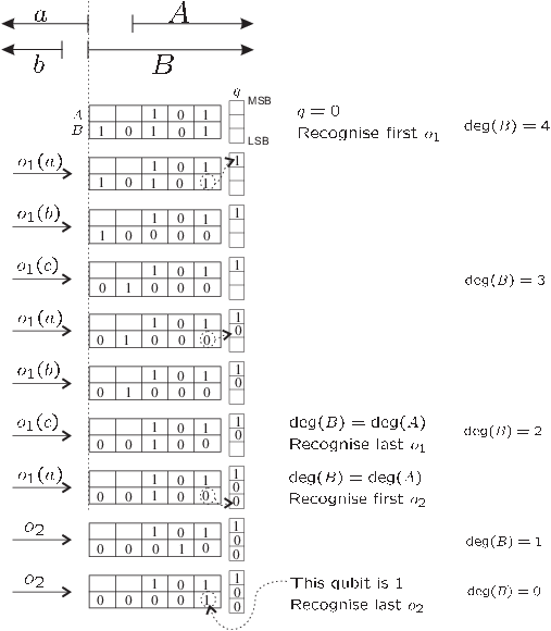
We have omitted the details of how to condition the steps of the long division on the value which determines the boundary for register sharing. For example, in the implementation of $A,B,0\leftrightarrow A,B+qA,q$ , the operations on $A,B,q$ will be conditioned on the value in the register containing $\deg(a)$ (from which the boundary position for register sharing can be determined). These details are very complicated, but the techniques for implementing controlled-gates in [BBC+95] indicate that it can be done with no ancillary qubits, and a polynomial increase in time.

8.2 Qubit space complexity

We saw in Section 4 that the number of qubits required to implement the elliptic curve group operation is bounded by the number of qubits required to implement the extended Euclidean algorithm for polynomials. Here we count the number of qubits required by our implementation.

By using register sharing, the values of $A,B,a,b$ can be stored using $2m$ qubits. The values of $\deg(A),\deg(B),\deg(a),\deg(b)$ must be initially computed and stored, requiring $4\left\lceil\log{m}\right\rceil+4$ qubits (as seen in Section 6.1). We also need to store the value of the quotient $q$ . We noted that in the extended Eulcidean algorithm for polynomials large quotients are rare. In [PZ03] it is shown that by bounding the size of $q$ to $3\left\lceil\log m\right\rceil$ bits, the total loss of fidelity will be at most $\frac{12}{m}$ , which is acceptable in the context of Shor’s algorithm. So we store $q$ in a register of $3\left\lceil\log m\right\rceil$ qubits.

For the synchronization we need a flag qubit $f$ , and 2-qubit counter register $c$ (to index the 4 operations $o_{1}(a),o_{1}(b),o_{1}(c),$ and $o_{2}$ used in the synchronization). Recall that we also need a “halting counter”, as the computations in the superposition will finish the extended Euclidean algorithm for polynomials after different numbers of iterations. The exact size of this halting counter depends on the exact time complexity of the algorithm. However, as our implementation is clearly polynomial in $m$ , we know that the size of the halting counter will be at most logarithmic in $m$ . We will write $H$ for the number of qubits required for the halting counter, where it is understood that $H$ is $O(\log m)$ . Such a halting counter would be required in any quantum implementation of the extended Euclidean algorithm for Polynomials.

So we have that the qubit space complexity for our implementation of the extended Euclidean algorithm for polynomials, and thus of the elliptic curve group operation for curves over $\textnormal{GF}(2^{m})$ , is

		$\displaystyle\underset{A,B,a,b}{\underbrace{2m}}+\underset{q}{\underbrace{3\left\lceil\log m\right\rceil}}+\underset{\deg{A},\deg{B},\deg{a},\deg{b}}{\underbrace{4\left\lceil\log{m}\right\rceil+4}}+\underset{f,c}{\underbrace{1+2}}+H$
		$\displaystyle=2m+7\left\lceil\log{m}\right\rceil+7+H.$

Acknowledgements

This research was supported by MITACS (Mathematics of Information Technology and Complex Systems), NSERC (National Science and Engineering Research Council), CSE (Communications Security Establishment), CSI (Canadian Foundation for Innovation), ORCDF (Ontario Research and Development Challenge Fund), and PREA (Premier’s Research Excellence Awards).

References

[BBC+95] A. Barenco, C.H. Bennett, R. Cleve, D.P. DiVincenzo, N. Margolus, P. Shor, T. Sleator, J. Smolin, H. Weinfurter, “Elementary gates for quantum computation”, Phys. Rev. A, 52:3457-3476, 1995.
[BBF03] Stephane Beauregard, Gilles Brassard, Jose Manuel Fernandez, “Quantum Arithmetic on Galois Fields”, Quant-ph/0301163.
[GN95] R.B. Griffiths, C.S. Niu, “Semiclassical Fourier Transform for Quantum Computation”, Phys. Rev. Lett. 76 (1996) pp. 3228-3231.
[HMV] D. Hankerson, A. Menezes and S. Vanstone, “Guide to Elliptic Curve Cryptography”, Springer-Verlag, 2003.
[Sho94] Peter Shor, “Algorithms for Quantum Computation: Discrete Logarithms and Factoring”, Proceedings of the 35th Annual Symposium on Foundations of Computer Science (1994), 124-134.
[VBE95] V. Vedral, A. Barenco, A. Ekert, “Quantum networks for elementary arithmetic operations”, Phys. Rev. A, 54, 147.
[PZ03] Christof Zalka, John Proos. “Shor’s discrete logarithm quantum algorithm for elliptic curves”, QIC Vol. 3 No. 4, pp 317-344 (2003), also quant-ph/0301141.

	$\displaystyle a$	$\displaystyle\rightarrow a^{\prime}=b+qa$
	$\displaystyle B$	$\displaystyle\rightarrow B^{\prime}=A.$

	$\displaystyle\deg(a^{\prime}B^{\prime})$	$\displaystyle=\deg((b+qa)A)$
		$\displaystyle=\deg(qaA)\hskip 14.22636pt\text{(since $\deg(qa)\geq\deg(a)>\deg(b)$)}$
		$\displaystyle=\deg(q)+\deg(a)+\deg(A)$
		$\displaystyle=\deg(B)-\deg(A)+\deg(a)+\deg(A)$
		$\displaystyle=\deg(aB)$
		$\displaystyle=m$