The Theory of Two-Photon Interference in an EIT System

Jianming Wen and Morton H. Rubin Email: rubin@umbc.edu Affiliation: Physics Department, University of Maryland, Baltimore County, Baltimore, MD 21250

August 11, 2026

Abstract

We examine the possibility of storing and retrieving a single photon using electromagnetically induced transparency (EIT). We consider the theory of a proof of principle two-photon interference experiment, in which an atomic vapor cell is placed in one arm of a two-photon interferometer. Since the two-photon state is entangled, we can examine the degree to which entanglement survives. We show that while the experiment might be difficult, it should be possible to perform. We also show that the two-photon interference pattern has oscillatory behavior.

pacs

42.50.Ct, 42.50.Dv, 42.50.Gy, 42.50.St

I Introduction

It is well-known that processes linear in the electromagnetic field have propagation properties that are independent of the strength of the field. This is part of the definition of linearity. In the quantum mechanical case, this is understood because the coupling between the electromagnetic field and matter is determined by the modes of the electromagnetic field independent of the state of the field, that is, independent of how the modes are populated. Consequently, the question of whether an experiment can be realized at the single photon level often reduces to a detailed analysis of the experiment. An example of this is the question of whether it is possible to coherently store and retrieve light at the single photon level. In this paper, we analyze this question by studying two-photon interference in which an atomic vapor cell is placed in one arm of the interferometer and the cell operated under the conditions of electromagnetically induced transparency (EIT) Harris; Mara; ScuZus.

The essence of EIT is to create destructive interference of the transitions for a three-level system in order to control the optical responses of the system. Harris et al. HFK first suggested how EIT can be used to slow the speed of light significantly compared with the vacuum case. Early experiments HauH; SL; Kash; BKRY on slow light have demonstrated that the group velocity $v_{g}$ can be reduced to several meters per second. The results reported in these experiments are based on the fact that EIT not only makes absorption zero at the resonant situation but also leads to a rapidly changing dispersion profile. The condition for slow light propagation leads to photon switching at an energy cost of one photon per event HarYama and to efficient nonlinear processes at energies of a few photons per atomic cross section HarHau.

Theoretically there are two ways to implement EIT. One way is adiabatic EIT Harris in which both the probe and coupling resonant lasers are adiabatically applied. After the system evolves into a steady state, EIT occurs for arbitrary intensities of the probe and coupling lasers. The other way is the transient-state EIT ScuZus, where resonant probe and coupling lasers are simultaneously applied. EIT occurs only when the intensity of the probe laser is much weaker than that of the coupling one.

In EIT the system is driven by two fields called the coupling and the probe, see Fig. 1 for notation. Most of the early theory and experiments of EIT took both coupling and probe lasers as classical external fields, see however Field. A disadvantage of the this approach is that it is hard to deal with atom-photon and photon-photon quantum entanglement which is of importance not only because of the interest of fundamental physics, but also for their potential applications to quantum computation and quantum communication NeilChuang. Recently a number of papers have treated the probe laser quantum mechanically FYL; FLukin.

In this paper we will take as the probe source a photon produced using spontaneous parametric down conversion (SPDC) Klyshko; Shih. In this nonlinear optical process a high-frequency photon is annihilated and two lower frequency photons, conventionally referred to as the signal and idler, are generated. The pair of photons are entangled in frequency and wave number. The correlations of the entangled two-photon system can be measured by means of coincidence counting detection. The purpose of the present paper is to study the optical properties of a transient-state EIT system interacting with one quantized field and investigate the response of the EIT medium to the nonclassical light field. We determine the two-photon interference in which one of the photons is stored and released. We want to examine whether the two-photon entangled state can be preserved in the process. There is an inherent mismatch of four orders of magnitude between the spectral bandwidth of SPDC and very narrow bandwidth of EIT; however, we shall see that it still may be possible to perform a proof of principle experiment.

This paper is organized as follows. In Sec. II, we discuss the quantum mechanical description of the system Hamiltonian. The equations of motion for the quantum probe field is given. In Sec. III, we investigate the optical properties of the EIT system related to the proposed experiment. In Sec. IV, the two-photon interference experiment of the correlated photon pairs generated by SPDC will be discussed when the signal photon is delayed in an EIT system. Finally, we summarize our results in Sec. V.

II Evolution of the operator

To describe the interaction of electromagnetic fields, the standard method is to start with the Bloch equations for the atomic density-matrix elements under the adiabatic assumption and moderate intensities of the fields. The equation of motion of the fields, which are treated as classical fields, are obtained from Maxwell equations. The detailed discussion can be found in FLukin; MLukin.

We consider a three-level atom with $\Lambda$ -type configuration interacting with two electromagnetic fields, which is shown in Fig. 1. The two lower metastable levels $|a\rangle$ and $|b\rangle$ are coupled to the upper excited level $|c\rangle$

Refer to caption — Figure 1: $\Lambda$ -type atomic configuration of EIT. The strong coupling field with frequency $\omega_{c}$ (Rabi frequency $\Omega_{c}$ ) resonantly drives the states $|b\rangle\rightarrow|c\rangle$ and the weak probe field with frequency $\omega_{p}$ (Rabi frequency $\Omega_{p}$ ) is applied to the states $|a\rangle\rightarrow|c\rangle$ with a small frequency detuning $\Delta$ , respectively. $\gamma_{c}$ and $\gamma_{b}$ are decay rates of states $|c\rangle$ and $|b\rangle$ .

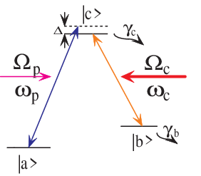
by the probe and coupling fields, with Rabi frequencies $\Omega_{p}$ and $\Omega_{c}$ , respectively. The coupling field is taken to be resonant $\omega_{cb}=\omega_{c},$ and the probe field is detuned by $\Delta=\omega_{ca}-\omega_{p}$ (see Fig. 1). In the interaction picture, the Hamiltonian of the system can be expressed as

\hat{H}=\hbar\left(\begin{array}[]{clrr}0&\Omega_{p}^{*}&0&\\ \Omega_{p}&\Delta-i\gamma_{c}&\Omega_{c}^{*}&\\ 0&\Omega_{c}&\Delta-i\gamma_{b}&\end{array}\right)

(1)

in the basis $\{|a\rangle,$ $|c\rangle,$ $|b\rangle\}.$ Assuming $|\Omega_{p}|<<|\Omega_{c}|$ , in the steady-state approximation, the eigenvalue of $\hat{H}$ associated with EIT is, to leading order in $|\Omega_{p}|^{2}$ ,

\zeta=-\hbar\frac{|\Omega_{p}|^{2}(\Delta-i\gamma_{b})}{(\Delta-i\gamma_{c})(\Delta-i\gamma_{b})-|\Omega_{c}|^{2}}

(2)

where $\zeta$ reduces to zero when $|\Omega_{p}|\rightarrow 0$ . This is the energy of the probe transition from the initially prepared atomic state $|a\rangle$ . The polarization of a medium with atomic density $N$ is the partial derivative of the interaction Hamiltonian with respect to the amplitude of the electric field, i.e.,

P=-N\langle\frac{\partial{H}}{\partial{E^{*}}}\rangle\ =-\frac{N\mu^{*}}{\hbar}\langle\frac{\partial{H}}{\partial{\Omega^{*}}}\rangle

(3)

where the second term comes from the definition of the Rabi frequency and $\mu$ is the electric dipole matrix element of corresponding transition.

In the weak-probe limit, the excited states will have a very small population, and the system evolves adiabatically so most of atoms are in the initially prepared state $|a\rangle$ . Under this condition, the interaction Hamiltonian $\hat{H}$ shown in Eq. (3) can be replaced by its eigenvalue, therefore,

P=-\frac{N\mu^{*}}{\hbar}\langle\frac{\partial{\zeta}}{\partial{\Omega^{*}}}\rangle.

(4)

From Eq. (2), one can obtain the polarization of the EIT medium at the probe frequency $\omega_{p}$ ,

P_{p}(\omega_{p})=\frac{N|\mu|^{2}}{\hbar}\frac{(\Delta-i\gamma_{b})}{(\Delta-i\gamma_{c})(\Delta-i\gamma_{b})-|\Omega_{c}|^{2}}E_{p},

(5)

and from $P_{p}=\epsilon_{0}\chi E_{p}$ , one finds the linear susceptibility,

\chi(\omega)=\frac{N|\mu|^{2}}{\hbar\epsilon_{0}}\frac{(\Delta-i\gamma_{b})}{(\Delta-i\gamma_{c})(\Delta-i\gamma_{b})-|\Omega_{c}|^{2}}.

(6)

This result can be found in ScuZus.

To quantize the probe field, we shall assume that the field is a quasi-monochromatic wave traveling in the $z$ -direction

\hat{E}_{p}=\sqrt{\frac{\hbar\omega_{p}}{2\epsilon_{0}V_{Q}}}\left(\hat{a}_{p}(t)e^{i(k_{p}z-\omega_{p}t)}+\hat{a}_{p}^{\dagger}(t)e^{-i(k_{p}z-\omega_{p}t)}\right).

(7)

One can introduce the effective Hamiltonian operator which describe the interaction between the fields and the EIT medium:

\hat{H}_{eff}=\frac{\hbar\omega_{p}}{2}\chi\hat{a}_{p}^{\dagger}(t)\hat{a}_{p}(t).

(8)

The evolution of the annihilation operator $\hat{a}_{p}$ is given by

\frac{\partial\hat{a}_{p}}{\partial t}=-i\frac{\omega_{p}}{2}\chi[\hat{a}_{p}^{+}\hat{a}_{p},\hat{a}_{p}]+\hat{F}=i\frac{\omega_{p}}{2}\chi\hat{a}_{p}+\hat{F}

(9)

where we must include the noise operator $\hat{F}$ ScuZus. Since it will not contribute to the counting rates, we will drop it. If the interaction starts at $t=0$ , field at the output of the EIT cell is given by

\hat{a}_{p}^{(out)}(t)=e^{-\frac{\chi^{\prime\prime}\omega_{p}t}{2}}e^{i\frac{\chi^{\prime}\omega_{p}t}{2}}\hat{a}_{p}^{(in)}(0)

(10)

where we have written $\chi=\chi^{\prime}+i\chi^{\prime\prime}$ in terms of its real and imaginary parts $\chi^{\prime}$ and $\chi^{\prime\prime}$ , respectively. The imaginary part of the susceptibility describes the amplitude change and the real part of the susceptibility gives the phase shift of the operator. Using $t=z/c$ Eq. (10) can also be written as

\hat{a}_{p}^{(out)}(z)=T\hat{a}_{p}^{(in)}(0)

(11)

where

T=e^{-\frac{\chi^{\prime\prime}\omega_{p}z}{2c}}e^{i\frac{\chi^{\prime}\omega_{p}z}{2c}}=e^{-\frac{\chi^{\prime\prime}\omega_{p}t}{2}}e^{i\frac{\chi^{\prime}\omega_{p}t}{2}}

(12)

is the transmission coefficient for the vapor.

III SPDC in EIT

SPDC has been studied for many years Klyshko; Shih; SPDC; ShihAlley; Shih1; Todd; Stre; Rubin; Rubin1. In this section we shall revisit type-II SPDC, paying particular attention to the passage of the beams through optical devices and the detection of the photons. We will consider both the single-photon counting detection and two-photon coincidence counting detection.

III.1 Single-Photon Detection of SPDC in EIT Medium

To fix notation we first discuss the single-photon properties of the radiation. Consider the experiment illustrated in Fig. 2, a monochromatic laser beam (pump beam with frequency $\omega_{pump}$ ) incident on a noncentrosymmetric birefringent crystal (e.g. BBO) produces pairs of photons. In Fig. 2 the point detector D detects the signal beam after EIT medium.

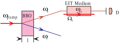
The average single-photon counting rate at detector D with efficiency $\eta$ is given by:

R_{s}=\eta\int\limits_{0}^{T}{dt_{s}}\langle\Psi|\hat{E}_{s}^{(-)}\hat{E}_{s}^{(+)}|\Psi\rangle

(13)

The field $\hat{E}_{s}^{(+)}$ is the positive frequency part of the signal field evaluated at the position $\vec{r}_{s}$ and the time $t_{s}$ and $\hat{E}_{s}^{(-)}$ is its Hermitian conjugate. $|\Psi\rangle$ is the state of the system at the output surface of the crystal. Generally $|\Psi\rangle$ is a superposition of the vacuum state $|0\rangle$ and states with any number of pairs of photons. Because of the small nonlinearity of the crystal, the expansion of $|\Psi\rangle$ in the perturbation theory is limited to the first two terms,

|\Psi\rangle=|0\rangle+\sum\limits_{\vec{k}_{s},\vec{k}_{i}}\Pi(\vec{k}_{s},\vec{k}_{i})\hat{a}_{s}^{+}(\vec{k}_{s})\hat{a}_{i}^{+}(\vec{k}_{i})|0\rangle

(14)

where $\vec{k}_{s}$ and $\vec{k}_{i}$ are the wave vectors of the signal and idler inside the crystal and $\hat{a}_{j}^{+}$ ( $j=s,i$ ) is the creation operator at the surface of the crystal. $\Pi(\vec{k}_{s},\vec{k}_{i})$ is the spectral function of the two-photon state determined from phase matching. The general form of the spectral function is

\Pi(\vec{k}_{s},\vec{k}_{i})=F(W_{s},W_{i})\Phi(\nu DL)h_{tr}(\vec{q}_{s},\vec{q}_{i})\delta(\omega_{s}+\omega_{i}-\omega_{p})

(15)

where

D=\frac{1}{v_{s}}-\frac{1}{v_{i}},

(16)

is the difference of inverse group velocities of the signal and idler, and the Dirac $\delta$ function arises from the steady-state or frequency phase-matching condition. The phase matching condition in the transverse direction is determined by the function $h_{tr}(\vec{q}_{s},\vec{q}_{i})$ where $\vec{q}_{s}$ and $\vec{q}_{i}$ are the transverse components of wave vectors of the signal and idler, respectively. The longitudinal phase matching condition gives $\Phi(\nu Dl)$ where $l$ is the length of the crystal and $\nu$ $=\omega_{s}-\omega_{i}.$ Finally, all of slowly varying variables are absorbed into $F(W_{s},W_{i})$ and $W_{s}$ and $W_{i}$ are the central frequencies of the signal and idler.

For simplicity, the following discussions are focused on the collinear case of degenerate type-II SPDC, i.e., the propagation along $z$ axis and $W_{s}=W_{i}=\omega_{p}/2$ . In this special case, the state of the system takes the form of Shih

|\Psi\rangle=\int{d\omega_{s}d\omega_{i}}\Phi(\nu Dl)\delta(\omega_{s}+\omega_{i}-\omega_{p})\hat{a}_{s}^{+}\hat{a}_{i}^{+}|0\rangle

(17)

with the phase matching function

\Phi(\nu Dl)=\frac{1-e^{i\nu DL}}{i\nu Dl}.

(18)

Note here we ignore all of constants and slowly varying variables in Eq. (17).

For the CW pump case considered here the single-photon counting rate is constant and is given by

R_{s}=\eta\int{d\nu}|\Phi(\nu Dl)T|^{2}=\eta\int{d\nu}S(\nu)

(19)

where $T$ is the transmission coefficient (Eq. 12),

S(\nu)=S_{0}(\nu)e^{\frac{\chi^{\prime\prime}\omega_{p}L}{v_{g}}},

(20)

and the unfiltered spectral function is

S_{0}(\nu)=\text{sinc}^{2}(\frac{\nu Dl}{2}).

(21)

The comparison between these two cases is illustrated in Fig. 3.

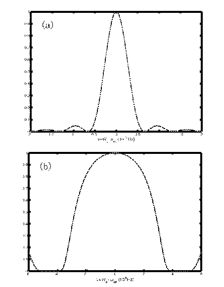
Note here that there are two frequency differences: one is coming from the non-perfect phase matching condition of SPDC, $\nu,$ and the other is from frequency detuning of the signal field in the EIT medium, $\Delta=W_{s}+\nu-\omega_{ac}$ . In Fig. 3 $S_{0}(\nu)$ and $S(\nu)$ are plotted. Note the different scales, from which we see that the dominate effect is the EIT absorption profile. The two sharp ”dips” are the signature of EIT phenomena, and correspond to two absorption peaks of the EIT medium. The interval between those two dips is proportional to the bandwidth of transparency window. If the central frequency of the signal beam does not coincide with the atomic transition rate, $W_{s}\neq\omega_{ac}$ , the spectrum distribution becomes asymmetric and the central peak will shift to left or right, which is determined by the larger one between $W_{s}$ and $\omega_{ac}$ . In order to prevent the bulk of the signal photons from obscuring the EIT signal it would be necessary to filter the beam using a narrow filter at the input of the cell.

III.2 Two-Photon Interference of SPDC in EIT Medium

In order to measure the two-photon correlation let us consider the simplified experiment shown in Fig. 4 ShihAlley. The entangled signal and idler photon pair emitted in the SPDC process is mixed by a 50-50 beam splitter (BS) and then recorded by photodetectors D1 and D2 for coincidence. In the idler channel, a time-delay apparatus ( $\delta\tau$ ) is put to balance the signal and idler path-lengths.

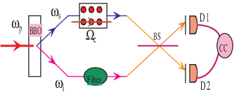
The two-photon coincidence counting rate is defined as Klyshko; Shih:

	$\displaystyle R_{cc}$	$\displaystyle=$	$\displaystyle\eta^{2}\frac{1}{T}\int\limits_{0}^{T}{dt_{1}}\int\limits_{0}^{T}{dt_{2}}\langle\Psi\|\hat{E}_{1}^{(-)}\hat{E}_{2}^{(-)}\hat{E}_{2}^{(+)}\hat{E}_{1}^{(+)}\|\Psi\rangle$		(22)
		$\displaystyle=$	$\displaystyle\eta^{2}\frac{1}{T}\int\limits_{0}^{T}{dt_{1}}\int\limits_{0}^{T}{dt_{2}}\|\Psi(t_{1},t_{2})\|^{2},$		(22)

where

\Psi(t_{1},t_{2})=\langle 0|\hat{E}_{1}^{(+)}\hat{E}_{2}^{(+)}|\Psi\rangle

(23)

is the effective two-photon amplitude. Taking into account the EIT cell, the two-photon amplitude is

\Psi(t_{1},t_{2})=\int{d\nu}\Phi(\nu Dl)Te^{-i(W_{s}+\nu)t_{1}}e^{-i(W_{i}-\nu)t_{2}}

(24)

As a comparison, the two-photon amplitude without an EIT medium is given by:

\Psi_{0}(t_{1},t_{2})=\int{d\nu}\Phi(\nu Dl)e^{-i(W_{s}+\nu)t_{1}}e^{-i(W_{i}-\nu)t_{2}}.

(25)

The coincidence counting rate for type-II SPDC now can be evaluated

$\displaystyle R_{cc}$	$\displaystyle=$	$\displaystyle\eta^{2}\int{d\nu}\{\|\Phi(\nu Dl)T(\nu)\|^{2}-Re[\Phi^{*}(\nu Dl)$	(26)
		$\displaystyle\times\Phi[(W_{i}-W_{s}-\nu)Dl]T^{*}(\nu)T(W_{i}-W_{s}-\nu)$
		$\displaystyle\times e^{-i(W_{s}-W_{i}+2\nu)\delta\tau}]\}.$

In the following discussions, we concentrate on the degenerate type-II SPDC, then the counting rate becomes

	$\displaystyle R_{cc}$	$\displaystyle=$	$\displaystyle Re\eta^{2}\int{d\nu}\text{ sinc}^{2}(\frac{\nu Dl}{2})\times[\|T(\nu)\|^{2}-T^{*}(\nu)T(-\nu)e^{i\nu(Dl-2\delta\tau)}]$		(27)
		$\displaystyle=$	$\displaystyle\eta^{2}\int{d\nu}\text{ sinc}^{2}(\frac{\nu Dl}{2})e^{-\frac{\chi^{\prime\prime}\omega_{s}L}{c}}\times\{1-\cos[\nu(Dl-2\delta\tau)-2\phi_{d}]\}.$		(27)

where $\phi_{d}(\nu)=\chi^{\prime}W_{s}L/2c$ , with $L$ the length of the EIT cell, is the phase delay of a pulse due to the EIT. We have assumed that the dispersion in the fiber can be ignored. For conventional two-photon interference experiments, removing the EIT medium in the signal channel, the coincidence counts of degenerate type-II SPDC read

R_{cc}^{(0)}=\eta^{2}\int{d\nu}|\Phi(\frac{\nu Dl}{2})|^{2}[1-\cos\nu(Dl-2\delta\tau)]

(28)

For simplicity, we assume perfect detection of photodetectors and ignored other losses, i.e., taking $\eta=1$ in the following discussions.

The comparison of coincidence counting rates between with the EIT medium and without it is shown in Fig. 5, again note the different frequency scales.

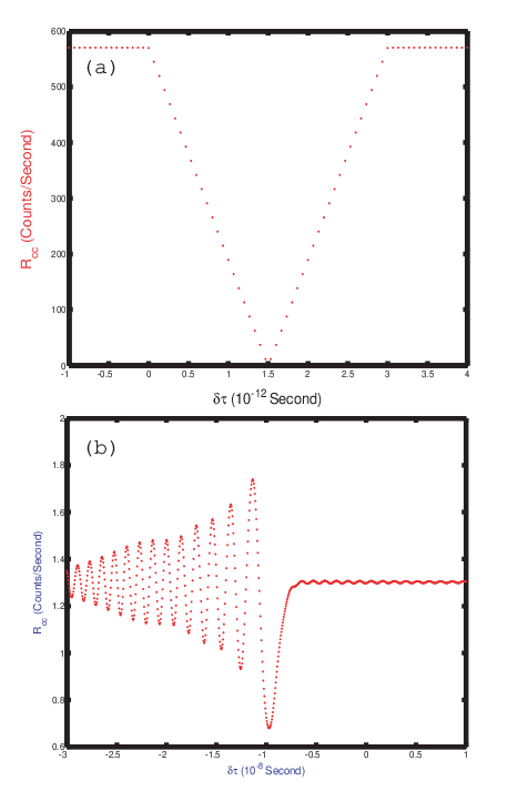
The quantum coherence from SPDC process still exists as is evident from Fig. 5 (b) where we see that in addition to a dip, there is an oscillation. The dip profile is much narrower than the notch shown in Fig. 5 (a) with no EIT cell. Recall that the center of the notch for the conventional coincidence counts is determined by $Dl/2$ , and its width is determined by the quantity $Dl$ (Eq. (28)). In Fig. 5(b), the dip center is displaced from $Dl/2$ by the time delay $\tau_{d}$ caused by EIT effect. The oscillations can be understood as follows. For the calculation of the figure we chose the special case that the center frequency of the signal beam coincides with the atomic transition rate, i.e., $W_{s}=\omega_{ca}$ . The transmission peak has a width of the $\Delta\omega_{tr}$ and is centered on $\nu=0.$ If $\Delta\omega_{tr}\times(Dl-2\phi^{\prime}_{d}-2\delta\tau)>1$ oscillations can occur while for $\Delta\omega_{tr}\times(Dl-2\phi^{\prime}_{d}-2\delta\tau)<1$ , where $\phi_{d}^{\prime}=d\phi_{d}/d\nu$ they will disappear. For the parameters used here, the width of transparency window is $\Delta\omega_{tr}=5.527\times 10^{9}Hz$ , the group velocity of single photons in the EIT medium is $v_{g}=1.064\times 10^{7}m/s$ , and the corresponding time delay is $\tau_{d}=9.069\times 10^{-9}Sec$ , so if $\delta\tau$ is negative we can get oscillations in the counting rate. In addition, because the transparency bandwidth of EIT is much narrower than the bandwidth of SPDC, the coincidence counting rate with an EIT medium (Fig. 5 (b)) is much lower than the conventional case. For the parameters given above, ignoring losses, the coincidence counts are around one photon per second, which is barely doable in the lab.

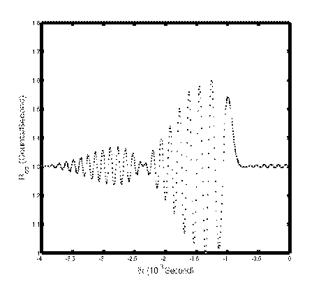
In Fig. 5(b) the dip center coincides with the time delay $\tau_{d}$ because of EIT dominant effect. If we do not use the resonant condition for the probe $W_{s}=\omega_{ca}$ , the visibility of coincidence counts is lowered and meanwhile the oscillations are modulated by the frequency mismatching (see Fig. 6). The visibility can be enhanced or decreased depending on the sign and magnitude of that frequency mismatching.

IV Conclusion

In this paper we present the methods to consider light storage at a single-photon level. The relation between the input and output field operator with an EIT medium is derived. Based on this relationship, the non-classical light (SPDC) storage is studied. We focused on the discussions about single-photon counts and two-photon coincidence counts of degenerate type-II SPDC with an EIT medium in slow light case. Though the experiment may be hard to implement, it is doable depending on the choice of experimental parameters. The results we have obtained are corresponding to the assumption that the coupling field is not a function of time.

Acknowledgements.

We would like to thank Michael Steiner for pointing out the importance of filtering the input beam. We also thank Prof. Yanhua Shih, the members of Quantum Optics Group at UMBC, and our collaborators at NRL for useful discussions. This work was partly supported by NRL through Grant No. code 5312.

References

(1) S. E. Harris, Physics Today 50 (7), 36 (1997).
(2) J. Marangos, J. Mod. Opt. 45, 471 (1998).
(3) M. O. Scully, M. S. Zubairy, Quantum Optics, Cambridge Univ., Cambridge (1997).
(4) S. E. Harris, J. E. Field, A. Kasapi, Phys. Rev. A 46, R29 (1992).
(5) L. V. Hau, S. E. Harris, Z. Dutton, C. H. Behroozi, Nature (London) 397, 594 (1999).
(6) S. Inouye, R. F. Low, S. Gupta, T. Pfau, A. Gorlitz, T. L. Gustavson, D. E. Pitchard, W. Ketterle, Phys. Rev. Lett. 85, 4225 (2000).
(7) M. M. Kash, V. A. Sautenkov, A. S. Zibrov, L. Hollberg, G. R. Welch, M. D. Lukin, Y. Rostovtsev, E. S. Fry, M. O. Scully, Phys. Rev. Lett. 82, 5229 (1999).
(8) D. Budker, D. F. Kimball, S. M. Rochester, V. V. Yashchuk, Phys. Rev. Lett. 83, 1767 (1999).
(9) S. E. Harris, Y. Yamamoto, Phys. Rev. Lett. 81, 3611 (1998).
(10) S. E. Harris, L. V. Hau, Phys. Rev. Lett. 82, 4611 (1999).
(11) J. E. Field and A Imamoglu, Phys. Rev. A 43, 2486 (1993); J. E. Field, Phys. Rev. A 47, 5064 (1993); M. Fleischhauer, Phys. Rev. Lett. 72, 989 (1994).
(12) M. A. Nielsen, I. L. Chuang, Quantum Computation and Quantum Information, Cambridge Univ., England (2000).
(13) M. Fleischhauer, S. F. Yelin, M. D. Lukin, Opt. Comm. 179, 395 (2000).
(14) M. Fleischhauer, M. D. Lukin, Phys. Rev. Lett. 84, 5094 (2000); M. Fleischhauer, M. D. Lukin, Phys. Rev. A 65, 022314 (2002),
(15) M. D. Lukin, Rev. Mod. Phys. 75, 457 (2003).
(16) D. N. Klyshko, Photons and Nonlinear Optics, Gordon and Breach Science Publishers, New York (1988).
(17) Y. H. Shih, Rep. Prog. Phys. 66, 1009 (2003).
(18) Y. H. Shih, A. V. Sergienko, M. H. Rubin, T. E. Kiess, C. O. Alley, Phys. Rev. A 49, 4243 (1994); ibid 50, 23 (1994); X. Y. Zou, L. J. Wang, L. Mandel, Phys. Rev. Lett. 67, 318 (1991).
(19) Y. H. Shih, C. O. Alley, Phys. Rev. Lett. 61, 2921 (1988), C. K. Hong, Z. Y. Ou, and L. Mandel, Phys. Rev. Lett. 59, 2044 (1987).
(20) Y. H. Shih, Adv. Atom. Mol. Opt. Phys., ed. B. Bederson and H. Walther, Academic Press, Cambridge (1997).
(21) T. B. Pittman, Two-Photon Quantum Entanglement From Type-II Spontaneous Down-Conversion, PhD Thesis, UMBC (1996).
(22) D. V. Strekalov, Biphoton Optics, PhD Thesis, UMBC (1997).
(23) M. H. Rubin, D. N. Klyshko, Y. H. Shih, A. V. Sergienko, Phys. Rev. A 50, 5122 (1994).
(24) M. H. Rubin, Phys. Rev. A 54, 5349 (1996).