Quantum Positioning SystemPreprint: v65
Abstract
A quantum positioning system (QPS) is proposed that can provide a user with all four of his space-time coordinates. The user must carry a corner cube reflector, a good clock, and have a two-way classical channel of communication with the origin of the reference frame. Four pairs of entangled photons (biphotons) are sent through four interferometers: three interferometers are used to determine the user’s spatial position, and an additional interferometer is used to synchronize the user’s clock to coordinate time in the reference frame. The spatial positioning part of the QPS is similar to a classical time-of-arrival (TOA) system, however, a classical TOA system (such as GPS) must have synchronized clocks that keep coordinate time and therefore the clocks must have long-term stability, whereas in the QPS only a photon coincidence counter is needed and the clocks need only have short-term stability. Several scenarios are considered for a QPS: one is a terrestrial system and another is a space-based-system composed of low-Earth orbit (LEO) satellites. Calculations indicate that for a space-based system, neglecting atmospheric effects, a position accuracy below the 1 cm-level is possible for much of the region near the Earth. The QPS may be used as a primary system to define a global 4-dimensional reference frame.
pacs
06.30.Ft, 06., 95.55.Sh, 42.50.DvI Introduction
During the past several years, the Global Positioning System (GPS) has practically become a household word. The GPS is a U.S. Department of Defense satellite system that is used by both the military and civilians for navigation and time disseminationParkinsonSpilker1996; Kaplan96; Hofmann-Wellenhof93. Automobile, ship, aircraft, and spacecraft use the GPS for navigation. Telephone and computer network systems that require precise time use the GPS for time synchronization. The GPS is a complex system consisting of approximately 24 satellites orbiting the Earth in circular orbits at approximately 4.25 Earth radii. The GPS is designed so that signals travel line-of-site from satellite to user, and from any place on Earth at least four satellites are in view. If a user receives four GPS satellite signals simultaneously from four satellites, , and the satellites’ space-time coordinates at time of transmission are known, the user can solve for his unknown space-time coordinates, , by solving the four equationsBahder2001; Bahder2003
| (1) |
In Eq.(1) we assume that the signals travel on four light cones that are centered at the reception event and we have ignored atmospheric delays. The actual signals that the GPS satellites transmit are continuous-wave circularly polarized radio-frequency signals on two carrier frequencies in the L-band centered about: MHz and MHz. The carrier frequency signals are modulated by a pseudorandom noise (PRN) code. A GPS receiver makes a phase difference measurement, called a pseudorange measurement, which is the phase difference between the PRN code received from the satellite and an identical copy of the PRN code that is replicated inside the GPS receiver, see Ref.Bahder2003 for details of the GPS pseudorange measurement process. The pseudorange measurement is essentially made by performing a correlation of the code bits in the PRN code received from the satellite with an identical copy of the same PRN code replicated inside the GPS receiver.
Recently, there have been several proposals for synchronizing clocks by making use of entangled quantum systemsChuang2000; Jozsa2000; Giovannetti2001; Giovannetti2001b; Giovannetti2002; Bahder2004; Shih2003. The question naturally arises whether entangled quantum systems can be exploited to determine all four space-time coordinates of a user, rather than just time.
In this article, I describe a quantum positioning system (QPS) that is in-principle capable of providing a user with all four of his space-time coordinates. This QPS is the quantum analog of the classical GPS described above. The QPS is based on entangled photon pairs (biphotons) and second order correlations within each pair. The two-photon coincidence counting rate is the basic measured quantity. In order to determine his four space-time coordinates, a user of the QPS must carry a corner cube reflector, a good clock, and have a two-way classical channel for communication with the origin of the reference frame.
II Interferometric Quantum Positioning System
For simplicity of discussion, I assume that space-time is flat with MinkowskiBahder2003 coordinates and that the user of the QPS is stationary. The complete QPS consists of four biphoton sources (entangled photon pairs), four beam splitters and four two-photon coincidence counting Hong-Ou-Mandel (HOM) interferometers, see Figure 1. Three of the interferometers are used together to solve for the user’s position and one interferometer is used to solve for the user’s time, in a particular reference frame.
Six spatial points, , where , for , define the spatial part of the reference frame at constant coordinate time . The six points define three independent baselines in pairs, , , and . The points are assumed to be accurately surveyed, so their coordinates are precisely known. Determination of a user’s spatial coordinates, , is done with respect to this reference frame. A stationary clock in this reference frame, say at the origin of coordinates, , provides a measure of coordinate time in this 4-dimensional system of coordinates. We neglect all gravitational effectsBahder2001 so that the user’s clock, which keeps proper time , runs at the same rate as coordinate time in the reference frame defined by the spatial points , so that . Synchronization of the user’s clock to coordinate timeBahder2004b means that we have a method to compute the integration constant in . In four dimensional flat space-time, the world lines of the spatial points define a tube. Events that are simultaneous in this system of 4-dimensional coordinates occur at constant values of coordinate time , which is a hyperplane that cuts this tube.
There are several possible modes for the QPS. First, consider a user that must determine all four of his space-time coordinates . In a previous paperBahder2004, an algorithm has been given to synchronize the proper time on a user’s clock to coordinate time, , without prior knowledge of the geometric range from the reference clock (which keeps coordinate time ) to the user clock. We assume that this algorithm is employed here to synchronize the user’s clock with coordinate time . This algorithm requires a two-way classical channel of communication between the user and the reference frame origin, where coordinate time is kept. The three spatial coordinates are determined separately as follows, refer to Figure 1.
Each baseline, such as the one connected by points, , contains an entangled photon pair (biphoton) sourceBurnham1970; HOM1987; Ghosh1986; KlyshkoBook1988; Rubin1994 located in the baseline. For convenience, we take the biphoton source to be at the midpoint of the baseline at point at position . Additionally, each baseline contains a 50:50 beam splitter and two photon detectors, see Figure 2. For simplicity of discussion, we assume that the biphoton source is essentially collocated with the beam splitter and two photon detectors at point , see Figure 2. Along the baseline there is a controllable optical delay at point . The other two baselines contain the same equipment, as shown in Figure 2. The QPS works as follows.
Photon pairs are created at , are sent to positions and , and are re-directed to the user at the unknown position . The two photon paths are similar, except that one path has a controllable optical delay . The optical delay is assumed to be calibrated so that we can accurately impose an arbitrary delay timedelaytime. Next, the entangled photons reflect from the user’s corner cube reflector at , and return back through the same paths, through points and , and arrive at a HOM interferometer that is collocated at at position , see Figure 2. For convenience, we assume that the interferometer is collocated with the photon generation point . Again, both photon return paths are similar, but one path has the optical delay . We have the following effective round-trip times for each photon path
| (2) | ||||
where is the geometric thickness of the optical delay perpendicular to the optical path and is the effective index of refraction for the optical delay . The optical delay is now adjusted until a minimum is observed in the two-photon counting rate at HOM1987. When the minimum in photon coincidence counting rate is observed at interferometer , the effective travel times for each photon path are equal, . The interferometer is balanced when the condition is satisfied, and a unique minimum is observed in the two-photon counting rate . The accuracy with which this minimum can be observed depends on the bandwidth of the band-pass interference filters used in front of the photon detectors.
We get an equation that relates the geometric path lengths to the measured optical delay time :
| (3) |
An analogous measurement process is carried out for the other two baselines. For simplicity, I assume that the points , , and are located at midpoints of their baselines. We then obtain the three equations
| (4) |
| (5) |
| (6) |
where for .
The two-photon coincidence counting rate is given byGlauber1965; Glauber1963; Mandel1995
| (7) |
where is the pump intensity in photons per second, and are the quantum efficiencies of detectors and , is a dimensionless constant and is the Fourier transform of the spectral function , which is the auotocorrelation function of the down-converted light
| (8) |
The Eqs.(4)-(6) can be solved for the three unknown user spatial coordinates, , in terms of the three measured time delays, , , , which balanced the three interferometers. The measured data consists of photon coincidence count rate vs. optical time delay lengths , for . Clearly a search must be done of the data to locate the minimum that corresponds to equal time of travel along the interferometer arms. The computations can be done at points , , and . This search to locate the minimum is the quantum analog of the correlation of the PRN code in a classical GPS receiver, which was described above. When the three interferometers at , , and have been balanced simultaneously, a classical message is sent to the user giving him the values of his coordinates . Clearly, classical communication is needed between the points , , and to establish that the interferometers are balanced at a given coordinate time . We imagine that when each interferometer is balanced, a message is sent to the origin of coordinates. When three messages are simultaneously received at the origin of coordinates (saying that the three interferometers are balanced), Eqs.(4)-(6) are solved for the user’s coordinates and the user’s coordinates are sent to the user through a classical channel of communication.
In the QPS that we describe, there is an apparent asymmetry in the determination of a user’s spatial coordinates, , and in the determination of the user’s time. In my view, this asymmetry is a reflection of the asymmetric way that space and time enter in the theory of the quantized electromagnetic field to give rise to photons as quanta of the field. As mentioned above, the time synchronization of the user’s clock to coordinate time is done by a method previously described by Bahder and GoldingBahder2004. Therefore in what follows, I discuss only the spatial part of the QPS.
With some modification of the above scheme, we may imagine that we could design a similar system based on first-order coherence for position determinationGlauber1965; Glauber1963. A single beam from a continuous-wave laser can be split and the beams sent on two different paths. However, in such a case, there would be an ambiguity that is associated with the wavelength of the light (interference fringes will be seen) that is unresolvable in principle. In contrast, in the quantum case (which relies on second-order coherence) the ambiguity is resolved because equal propagation times for two paths lead to quantum interference: equal travel times for two paths create a unique observable minimum in the two-photon coincidence counting rate .
The measured quantities in the QPS are the optical path delays . For a given measured value of optical delay, say , Eq.(4) specifies that the user’s coordinates must lie on a hyperboloid surface with foci at and , i.e., a hyperbola of revolution that is symmetric about the baseline defined by and . The user’s position, , is then given by the intersection of three hyperbolas given by Eq.(4)-(6). Each Eq.(4)-(6) is just the equation for a baseline in a classical time of arrival (TOA) system that records arrival times of classical light pulses (or distinct intensity edges) at two spatial reception points . In the case of a classical TOA system, pulse arrival time at four locations is needed to determine all four space-time coordinates. In that case, four time difference of arrival (TDOA) equations can be formed from four points, and each point is used multiply to (effectively) form the baselines. (Taking TDOAs results in a system of three equations where the emission event time has cancelled out. ) In the quantum case, since correlations between photon pairs are used, we must use three baselines defined by six points , plus an additional interferometer for the determination of the user’s time. As we will see below, the QPS is an interferometric system.
More fundamentally, and more significant for applications, is that in the classical case of a TOA system, we must have good clocks that are synchronized to coordinate time so that accurate pulse arrival times at the four reception points can be recorded. A good clock that keeps coordinate time is often a difficult requirement to meet in practiceclock stability. In contrast, in the quantum case two-photon coincidence counts at detectors and are measured and only a good ”flywheel” clock is needed (i.e., a clock having a good short-term stability) to measure photon coincidence count rates while the optical time delay is adjusted, to locate the minimum in .
III Geometric Dilution of Precision
In the case of the classical GPS, the geometrical positions of the GPS satellites determine the accuracy of the user’s position. This effect is sometimes called the geometric dilution of precision (GDOP). We compute the positioning accuracy and the effect of GDOP for the QPS from Eq.(4)-(6). These equations give an implicit relation for the user position as a function of the three measured path delays, , and the six baseline endpoints . If we knew the error in the measured path length delays, , and , we could compute the error in the three components of the user’s position vector, , from
| (9) |
for constant . However, these errors are statistical in nature, so instead I compute the standard deviations , , and , of the user coordinates , , and , as a function of the standard deviations , , and , of the measured optical time delays , , and . For constant for , these standard deviations are related byBevington2003
| (10) | ||||
where the partial derivatives are done at constant . The lengthy calculation to compute the partial derivatives in Eq.(10) is done analytically using Mathematica. For simplicity, I assume that the error distributions of the are Gaussian and that the three standard deviations are equal, . For a spherically symmetric probability distribution of 3-dimensional positions , the spherical error probable (SEP), which is the radius within which 50% of the points lie, is relatedBahder1995Rep to the standard deviations by . In our case, the probability distribution of is not necessarily spherical. To approximate the SEP error metric, we compute a weighted approximation to the SEP metric by defining . When the error distribution for is spherically symmetrical, the error metrics are equal: . I consider the effect of GDOP for two cases, one in which the interferometer baselines are near each other, and the other case where the baselines are well separated, which is the case with classical GPS or a classical TOA system.
III.1 Geodetic Positioning System
First, consider a case where the three baselines coincide with the three Cartesian coordinate axes of a reference frame, see Figure 3. Such a case might occur when the baselines are on the Earth, and we want to determine the position of an object with respect to a topocentric coordinate system. For example, consider the center of the QPS at the origin of Cartesian coordinates and an object with a corner reflector at a range of 100 from the QPS, with coordinates . Figure 4 shows a plot of contours of constant values of in the plane at , for the interferometer arm (half) length and error (standard deviation) in optical path . In the contour plot, the position error is for , whereas for the error , which corresponds to the upper right high-accuracy (light-shaded) region in Figure 4. On the -axis at and the error is essentially infinite. Figure 5 shows a plot of the error metric vs. , for and /, which corresponds to a line in Figure 4 with relatively small error . In the high-accuracy light-shaded region of Figure 4, for and /, the dependence of the error on the baseline length is plotted in Figure 6, also using . For a four-meter baseline, , the error is just under .
Note that the position error depends linearly on , which is the standard deviation (error) in measurement of the optical path delay needed to obtain the minimum in two-photon coincidence counts . The width of this minimum depends on the interference filters in front of the photon coincidence counting detectors as well as the pump laser bandwidthHOM1987; Grice1997. Depending on the experimental design, this minimum may be measured to better than , which was used in these plots, and hence accuracies may be better than plotted.
Finally, I note that the error function has a very complex dependence on user coordinates , and as stated earlier, the error function also depends critically on the way the baselines are distributed, i.e., it depends on the six points for , which define the baseline endpoints. In the next example, I consider a situation where the baselines do not intersect, and thereby the error is considerably smaller than for the case considered above, even though the distances are larger.
III.2 Satellite-based QPS
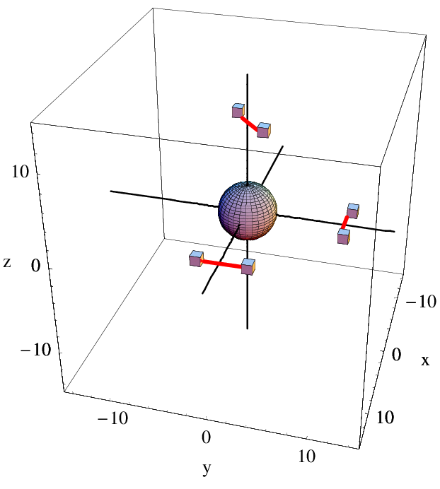
Now assume that each point of a baseline, , is associated with a different satellite, and that the spatial interferometer legs are formed from pairs of points , , and , see Figure 7. Specifically, I assume that the points , are on low-Earth orbit (LEO) satellites. It may seem optimistic that a QPS is feasible with such large baselines because single photons must be propagated over these baselines and then reliably detected. However, recently single photons have been propagated through the atmosphere and detected over 10 distance in daylightHughes2002, and another study concludes that there are no obstacles to create a single-photon quantum key distribution system between ground and low-Earth orbiting satellitesRarity2002 . Therefore, a LEO-satellite QPS may be possible.
As an example of the positioning errors in a QPS made from LEO satellites, I take the baseline endpoints to be: , , , , , and . A plot of this configuration is shown in Figure 7. A contour plot of the reciprocal error function, , is shown in the plane for , where is the Earth’s radius, see Figure 8. As an example, in the calculations below I take the semi-major axis of the LEO satellites to be and the baseline between pairs of satellites as . The standard deviation (error) in the measured optical delay is taken to be . For a user on the surface of the Earth with coordinates the error is For these same parameters, Figure 9 shows a plot of the position error vs. for . Note that over a large range of -values the error remains below . Finally, Figure 10 shows a plot of the position error in the radial direction: vs. for the same parameters. On a radial line in the (1,1,1) direction, the error remains below up to However, near the error rises steeply. This is an example of the complex dependence of on user position, which was mentioned earlier.
Clearly, the geometric positioning and layout of the baselines significantly affects the accuracy of a user’s position. Note that the terrestrial QPS (discussed in the previous section) had a ratio of baseline length to user position , whereas this LEO satellite QPS has . By comparing the baseline layout for the terrestrial QPS and this LEO satellite QPS, it is clear that the positioning accuracy is sensitive to the separation and layout of the baselines, but not so sensitive to the baseline lengths. Other calculations (not shown) support this conclusion.
The above calculations for a satellite-based QPS are only meant as an example to illustrate the magnitude of errors in position that may be achievable. A significant amount of engineering calculations must be performed to design a realist satellite-based QPS. Furthermore, real satellites are moving and engineering similar to that used in the classical GPS would have to be done, e.g., using Kalman filtering techniques. Obviously, bright sources of entangled photons (biphotons) are needed. The calculations above suggest that if properly engineered, a satellite-based QPS may achieve position accuracy of objects near the Earth’s surface below 1. In these calculations, I have ignored the time delays introduced by the atmosphere. However, corrections can be made for atmospheric effects using multiple colors of photons similarly to what is done with the GPS. Perhaps one advantage of the quantum system as compared to the classical GPS is that entangled photons exhibit group velocity dispersion cancellation, which may be an important factor for future engineering and design of a QPS Steinberg1992; Steinberg1992a; Perina1999; Valencia2002.
IV Alternative Scenarios
IV.1 Position-Only Determination
A QPS can be designed to work in several modes, depending on the needs of the user and the required scenario. In the above discussion, we have described the case where a user of the QPS wants to determine both his spatial and time coordinates, . A second alternative is that a user may only need to obtain their spatial coordinates, and he may not need the correct time. In this latter case, the time synchronization portion of the system is not needed, and the user may find their position coordinates by having only a corner reflector and a one-way (reception only) classical channel of communication with the reference frame origin, where the simultaneity of the three two-photon coincidence counting rate minima is established.
Another mode of operation of a QPS is where we want to determine the position of an object with a corner cube reflector, such as a geostationary satellite. In such a case, information on the position of the satellite, , is only needed on the ground. The satellite’s position coordinates can be determined on the ground using a QPS, and only a corner cube reflector is needed on the satellite, but no communication channel to the satellite and no on-board clock is needed.
IV.2 User Carries QPS Receiver
The scenarios that we have described above are ones where the measurements (adjusting the optical delays) and the calculations (to compute ) are done near the origin of the reference frame. In a classical GPS receiver, the computations (correlations of PRN codes to at least four satellites) are done locally in the user’s GPS receiver that the user carries with him. The QPS analog of this classical GPS scenario is a setup where the biphotons are generated at points , and , but the user carries with him the 50:50 beam splitters and photon detectors. In this scenario, the user controls (and carries with him) the optical delays, see Figure 1, and he locally measures the optical delays , and . The user must receive a classical message consisting of the coordinates of baseline endpoints, , , and then he must solve the Eq.(4)-(6) for his position . In such a case, there are no clocks on-board the broadcasting satellites (located at positions ), however, the user must carry a clock with short term stability to determine rate of photon coincidence counts from each of the three baselines (associated with spatial positioning) and also he must do coincidence counting for time determination (if time is needed). For the three spatial baselines, optical propagation is then one-way (using the satellite positions as a primary reference system, see below) from satellites to QPS user receiver. For time synchronization, however, as mentioned previously, the optical propagation must be two-way (when using the method of Bahder and Golding). In essence, for each of the four channels, the QPS receiver consists of a beam splitter, two single-photon detectors, and a controllable optical delay. All four space-time coordinates can be obtained by a user in this way. One clock in the reference frame must have long-term stability to define coordinate time, and another clock in the QPS user receiver can have short-term stability. Note that the satellites do not need to carry clocks, because their positions can be used to define the primary system of coordinates. This type of QPS is a close analog of the classical GPS.
V QPS Space-time Coordinates
The satellites at baseline points can be taken to define the primary system of reference, even though the points change with time. The quantities measured by a user of such a QPS are then , where is the optical time delay (in the HOM interferometer) that will provide the user with coordinate time in this coordinate system (using the Bahder and Golding method), and are the three optical delays in the three interferometers for position determination. The quantities are then to be regarded as generalized 4-dimensional space-time coordinatesSynge1960, is a time-like coordinate and are space-like coordinates. Within the context of general relativity, such coordinates are as good as any other coordinates, and they enter into the metric of the flat space-time assumed in this work. Of course, a transformation from the QPS space-time coordinates, , to an Earth-centered inertial (ECI) system of coordinates, say , is of interest for astrodynamic applications. Such a transformation can be done approximately by conventional means of tracking the satellites (at baseline points ).
It is interesting to remark that the QPS allows the direct measurement of 4-dimensional space-time coordinates. Previously, it was believed that space-time coordinates were not measurable quantitiesSynge1960; Pirani1957; Soffel1989; Brumberg1991. Of course, the QPS coordinates are real physical measurements, and it is well-known that real measurements are space-time invariants under generalized coordinate transformationsSynge1960.
VI Summary
I have presented a conceptual scheme for an interferometric quantum positioning system (QPS) based on second order quantum coherence of entangled photon pairs (biphotons). A user’s spatial coordinates are determined by locating three unique minima in three different two-photon counting rates, associated with three HOM interferometers built on independent baselines. The spatial portion of the QPS is similar to a classical TOA system, however, a classical TOA system requires synchronized clocks that keep coordinate time, which is often a difficult requirement to meet. In contrast, the QPS only requires a clock having a short-term stability to measure two-photon coincidence counting rates while the optical time delay is adjusted (to locate the minima in the two-photon coincidence counting rate ). Bright sources of entangled photons (biphotons) are needed.
Several different scenarios were considered for a QPS: one is a terrestrial system and the another is space-based. In both cases, I computed the accuracy of a user’s position as a function user position. The function that describes the errors in position has a complex spatial dependence. In the case of the terrestrial QPS, the position accuracy was relatively poor because the baselines were located near each other. This could be dramatically improved by moving apart the baselines.
As an example of a satellite-based QPS, I have proposed a LEO-satellite QPS. Neglecting atmospheric effects, calculations suggest that the position accuracy of such a QPS can be below the 1 cm-level for an error (standard deviation) in the optical delays associated with the minima in two-photon counting rates . The complex dependence of on user position suggests that significant engineering must be done to design a realistic QPS.
Acknowledgements.
This work was sponsored by the Advanced Research Development Activity (ARDA). The author is grateful to Yanhua Shih for helpful communications.References
- (1) Global Positioning System: Theory and Applications, Vols. I and II, edited by B. W. Parkinson and J. J. Spilker, Progress in Astronautics and Aeronautics, Vols. 163 and 164 Amer. Inst. Aero. Astro., Washington, D.C., 1996.
- (2) E. D. Kaplan, Understanding GPS: Principles and Applications, Mobile Communications Series (Artech House, Boston, 1996).
- (3) B. Hofmann-Wellenhof, H. Lichtenegger, and J. Collins, Global Positioning System Theory and Practice (Springer-Verlag, New York, 1993).
- (4) T. B. Bahder, Am. J. Phys. 69, 315, 2001, ”Navigation in curved space-time”.
- (5) T. B. Bahder, Phys. Rev. D 68, 063005 (2003).
- (6) I. L. Chuang, Phys. Rev. Lett. 85, 2006 (2000), and also in quant-ph/0004105.
- (7) R. Jozsa, D. S. Abrams, J. P. Dowling, and C. P. Williams, Phys. Rev. Lett. 85, 2006 (2000).
- (8) V. Giovannetti, S. Lloyd, and L. Maccone, Nature 412, 417 (2001).
- (9) V. Giovannetti, S. Lloyd, and L. Maccone, F. N. C. Wong, Phys. Rev. Lett. 87, 117902 (2001).
- (10) V. Giovannetti, S. Lloyd, and L. Maccone, Phys. Rev. A, 65, 022309 (2002).
- (11) Y. Shih, unpublished.
- (12) T. B. Bahder and W. M. Golding, “Clock synchronization based on second-order coherence of entangled photons”, submitted for publication in Phys. Rev. A , April 2004.
- (13) T. B. Bahder, ”Clock Synchronization and Navigation in the Vicinity of the Earth”, gr-qc/0405001, to be published in ”Progress in General Relativity and Quantum Cosmology Research”, Nova Science Publishers, Inc., Hauppauge, New York, December 2004.
- (14) D. C. Burnham and D. L. Weinberg, Phys. Rev. Lett. 25, 84 (1970).
- (15) C. K. Hong, Z. Y. Ou, and L. Mandel, Phys. Rev. Lett. 59, 2044 (1987).
- (16) R. Ghosh, C. K. Hong, Z. Y. Ou, and L. Mandel, Phys. Rev. A 34, 3962 (1986).
- (17) D. N. Klyshko, Photons and Nonlinear Optics (Gordon & Breach, New York, 1988).
- (18) M. H. Rubin, D. N. Klyshko, Y. H. Shih, and A. V. Sergienko, Phys. Rev. A 50, 5122 (1994).
- (19) This optical time delay can be a free-space delay, or it may be a high-index optical material medium, such as cold atoms, see for example: C. Liu, Z. Dutton, C. H. Behroozi, and L. V. Hau, ”Observation of coherent optical information storage in an atomic medium using halted light pulses”, Nature 409, 490 (2001).
- (20) R. J. Glauber, Optical Coherence and Photon Statistics, Lectures delivered at Les Houches during 1964 Summer School of Theoretical Physics at University of Grenoble, Gordon Breach Science Publishers, New York (1965).
- (21) R. J. Glauber, Phys. Rev. 130, 2529 (1963); Phys. Rev. 131, 2766 (1963)
- (22) L. Mandel and E. Wolf, ”Optical Coherence and Quantum Optics”, Cambridge Iniversity Press, New York (1995).
- (23) For example, the GPS satellite clocks (essentially) keep coordinate time and must have a good long-term stability, see Ref.Bahder2003.
- (24) P. R. Bevington and D. K. Robinson, ”Data Rediction for the Physical Sciences” McGraw-Hill, New York, (2003).
- (25) T. B. Bahder, ”GPS for Land Combat Applications”, Summary Report of the Army Workshop held at University of North Carolina, 2 and 3 August 1995, Army Research Laboratory Technical Report ARL-SR-40, December 1995.
- (26) W. P. Grice and I. A. Walmsley, Phys. Rev. A, 56, 1627 (1997).
- (27) R. J. Hughes, J. E. Nordholt, D. Derkacs and C. G. Peterson, New Journal of Physics 4, 43.1 (2002).
- (28) J. G. Rarity, P. R. Tapster, P. M. Gorman and P. Knight, New Journal of Physics 4, 82.1 (2002).
- (29) A. M. Steinberg, P. Kwiat, and R. Y. Chiao, Phys. Rev. A 45, 6659 (1992).
- (30) A. M. Steinberg, P. Kwiat, and R. Y. Chiao, Phys. Rev. Lett. 68, 2421 (1992).
- (31) J, Perina, A. Sergenko, B. M. Jost, B. E. A. Saleh, and M. Teich, Phys. Rev. A 59, 2359 (1999).
- (32) A. Valencia, M. Chekhova, A. Trifonov, and Y. Shih, Phys. Rev. Lett. 88, 183601 (2002).
- (33) J. L. Synge, Relativity: The General Theory, North-Holland, New York (1960).
- (34) A. E. Pirani, Bulletin De L’Academie Polonaise Des Sciences Cl. III, 1957, Vol. V, No. 2, p. 143-146 (1957).
- (35) M. H. Soffel, Relativity in Astrometry, Celestial Mechanics and Geodesy, Ch. 3, Springer-Verlag, New York (1989).
- (36) V. A. Brumberg, In section 2.3 of Essential Relativistic Celestial Mechanics, published under the Adam Hilger imprint by IOP Publishing Ltd, Techno House, Bristol, England (1991).
- (37) B. Guinot, Application of general relativity to metrology”, Metrologia 34, 261 (1997).