Bohmian transmission and reflection dwell times without trajectory sampling

For a 1D static detector located in the spatial interval $[a,b]$ (see figure 1), the average dwell time of an ensemble of quantum systems with wave function $\Psi$ from time $\tau_{i}$ up to time $\tau_{f}$ is generally agreed to be given by

$$\int_{\tau_{i}}^{\tau_{f}}dt\int_{a}^{b}d\xi\;\left|\Psi(t,\xi)\right|^{2},$$

(1)

cf the reviews [1]¹¹ 1 Clearly expression (1) does not exist for bound states.. It is motivated by classical reasoning [2], and it also has been derived within Bohmian mechanics [3]. In a recent work [4] a corresponding dwell time operator has been investigated.

Dwell times of the type (1) were associated with interaction times in collision processes long ago [5]. The relevance of these interaction times to time resolved scattering experiments has been studied, e.g., in [6]. Through these works it became clear, that differences of average dwell times formed between a scattering wave packet and its free incoming asymptote are measurable quantities.

With the introduction of the Larmor clock by Baz [7], dwell time expressions themselves have got measurable status. The idea is that a small and uniform magnetic field, which is confined to a small region of space, causes a Larmor-precession of the spin-polarization vector of the scattered wave. It was shown in [8] that the Larmor clock indeed reveals the average dwell time. If it also is capable of displaying the spectral distribution of some dwell time operator is still unclear.

The specialization of the Larmor clock to the case of one-dimensional scattering was done by Rybachenko in [9]. In this work (to the authors knowledge for the first time) a distinction into the dwell times of the finally transmitted respectively reflected partial waves has been introduced. For short such selective dwell times will further on be denoted as transmission and reflection times. Another approach to transmission and reflection times, grounded on a specific experimental scheme, was introduced by the oscillating barrier model of Büttiker and Landauer [10]. This model is widely believed to have ignited the tunnelling time controversy anew. A further extension of the Larmor clock by Büttiker [11] incorporates the effect of spin-alignment with the magnetic field.

More recently the interest in transmission times has been driven on the one hand by the very indirect time measurement techniques of the condensed matter community, especially in connection with tunnelling in semiconductor heterostructures or Josephson junctions. On the other hand, the progress in laser cooling techniques in quantum optics delivers another valuable tool for future time resolved scattering experiments.

It is no surprise that the detailed definition of transmission and reflection times depends on the situation under scrutiny. A systematic operator approach embodying several such possible definitions was given by Brouard et al [12]. It was shown, however, that transmission and reflection times derived within the framework of Bohmian mechanics are not included in this catalogue ([13], chapter 5).

Bohmian mechanics comprises the mathematical concept of world lines or trajectories and with this the term ‘particle’ obtains substance in quantum theory again. Thus the notion of dwell time can be addressed in a straightforward manner, very much like in classical mechanics. The dwell time of a particle in the spatial interval $[a,b]$ is simply defined as the duration during which the particle’s trajectory is localized within $[a,b]$. For an elaborate discussion of Bohmian mechanics see [14].

As the numerical effort involved with the calculation of Bohmian world lines is immense, there have been attempts to compute the Bohmian transmission and reflection times without the sampling of trajectories. A related one-dimensional bound-state situation has, e.g., been studied by Stomphorst in [15]. In the present paper a formulation without trajectories for the transmission and reflection times in a genuine scattering situation is presented. The derivation closely follows ideas developed for the treatment of 1D arrival time in [16]. As an application the scattering from a double potential barrier, reminiscent of semiconductor-heterojunctions in, e.g., resonant tunnelling diodes, is considered.

We consider a scattering situation in which the Møller operators $\Omega^{in}$ and $\Omega^{out}$ exist and are asymptotically complete [17]. $\Psi(t,\cdot)=e^{-iHt/\hbar}\Omega^{in}\phi_{0}=\Omega^{in}e^{-iH_{0}t/\hbar}\phi_{0}$ denotes the scattering solution with incoming asymptote $\phi(t,\cdot)=e^{-iH_{0}t/\hbar}\phi_{0}$. The solution $\phi(t,\cdot)$ of the free Schrödinger equation is chosen to be localized on the negative spatial semi-axis for $t\to-\infty$. That is the case if and only if the Fourier transform $\mathcal{F}(\phi_{0})$ is localized on the positive half-line [18].

The Bohmian transmission time in the above scattering situation is defined as follows. Let $\gamma_{x}(t)$ denote the Bohmian trajectory which at time $t=0$ passes through the point $x$. There exists a critical value $x_{c}\in\mathbb{R}$, such that $\lim\limits_{t\to\infty}\gamma_{x}(t)=-\infty$ for all $x<x_{c}$ and that $\lim\limits_{t\to\infty}\gamma_{x}(t)=\infty$ for all $x>x_{c}$. Therefore the Bohmian transmission time is defined as

$$\langle\tau_{T}\rangle=\int\limits_{-\infty}^{\infty}dx\;|\Psi(0,x)|^{2}\cdot\Theta(x-x_{c})\int\limits_{\tau_{i}}^{\tau_{f}}dt\;\chi_{[a,b]}(\gamma_{x}(t))$$

(2)

with $\chi_{[a,b]}$ the characteristic function on the interval $[a,b]$ and $\Theta$ the Heaviside step function. See, e.g., [19]. Analogously the reflection time $<\tau_{R}>$ is defined by replacing the term $\Theta(x-x_{c})$ in the right hand side of equation (2) by $\Theta(x_{c}-x)$. The critical trajectory $\gamma_{x_{c}}(t)$ ($\gamma_{x_{c}}(0)=x_{c}$) is implicitly defined by

$$|T|^{2}=\int_{\gamma_{x_{c}}(t)}^{\infty}|\Psi(t,\xi)|^{2}\;d\xi,\quad\forall t\in\mathbb{R}.$$

(3)

Thereby

$$|T|^{2}:=\lim_{t\to\infty}\int_{0}^{\infty}|\Psi(t,\xi)|^{2}\;d\xi$$

(4)

is the transmission probability of the scattering system. The lower limit of the integral in (4) can equally be replaced by any finite $q\in\mathbb{R}$. Accordingly by $|R|^{2}:=1-|T|^{2}$, the reflection probability is defined. Thus the conditional transmission respectively reflection times, i.e. transmission and reflection times normalized to the fraction of transmitted respectively reflected particles of the entire ensemble, are $<\tau_{T}>^{c}:=\frac{1}{|T|^{2}}<\tau_{T}>$ and $<\tau_{R}>^{c}:=\frac{1}{|R|^{2}}<\tau_{R}>$.

However, the calculation of Bohmian transmission and reflection times can be reduced to the computation of current density integrals along the edges at $x=a$ and $x=b$. The next proposition represents a generalization of expressions already proposed in [20].

As an example for a 1D scattering situation we consider the case of a Gaussian wave packet impinging on a double potential barrier, i.e. we are looking for solutions $\Psi$ to the Schrödinger equation

$$i\hbar\,\partial_{t}\Psi=\left[-\frac{\hbar^{2}}{2m}\partial_{x}^{2}+V\right]\Psi$$

with

$$V=V_{0}\cdot\chi_{[a,b]}+V_{1}\cdot\left(\chi_{[a^{\prime},a[}+\chi_{]b,b^{\prime}]}\right).$$

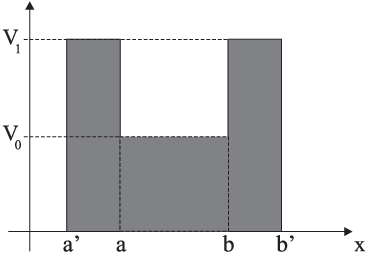
$\chi_{[\alpha,\beta]}$ denotes the characteristic function on the interval $[\alpha,\beta]\in\mathbb{R}$ and $a^{\prime}<a<b<b^{\prime}$ (see figure 2). The parameter reduction $\hbar,m,V_{0}\to 1$, e.g., is achieved by taking time in units of $\frac{\hbar}{2V_{0}}$, space in units of $\frac{\hbar}{\sqrt{2mV_{0}}}$. $V_{1}$ is taken in units of $V_{0}$. In figure 3(a) the evolution of the probability density $|\Psi|^{2}$ is given for the case $a^{\prime}=-6$, $a=-3$, $b=3$, $b^{\prime}=6$ and $V_{1}=2$ in the chosen units. The mean kinetic energy of the packet is $1.5^{2}V_{0}=2.25V_{0}$. In figure 3(b) a sample of 50 corresponding Bohmian trajectories is illustrated. The initial distribution of starting points of the trajectories resemble the initial Gaussian distribution of the wave packet. Figure 4 shows a zoom into the area indicated by the rectangle in figure 3(b).

Finally, in figure 6 the mappings $\mathcal{T}_{T}(s)$ (a), $\mathcal{T}_{R}(s)$ (b) and $\mathcal{T}_{D}(s)$ (c) are illustrated, which give the Bohmian transmission, reflection and overall average dwell times $<\tau_{X}>$, $X\in\{T,R,D\}$ in $[a,b]$ from time $\tau_{i}=0$ onwards as a function of the upper temporal bound $s=\tau_{f}$. In addition the conditional transmission and reflection times, i.e. normalized to the fraction of finally transmitted or reflected particles, are indicated in (a) and (b).

Introducing as parameters the potential energy $V_{0}=0.25$ eV (i.e. $V_{1}=0.5$ eV) and the effective electron mass $m_{*}=0.07m_{e}$ typical for $GaAs/GaAlAs$ double barrier heterostructures (see e.g. [22]), the temporal units get approximately $1.3$ fs, the spatial units approximately $15$ $\AA$. Therefore the width of the model heterostructure in figure 2 is in the range of $200$ $\AA$, which is easily achieved by the ultrathin layers of modern semiconductor devices.

I’m much indebted to Gebhard Grübl for helpful discussions and corrections and also to Peter Wagner for valuable suggestions regarding the appendix, both University of Innsbruck. This work has been supported by Doc-Fforte [Doctoral Scholarship Programme of the Austrian Academy of Sciences].

Recall that the scattering solutions under consideration are given by $\Psi(t,\cdot)=\Omega^{in}\phi(t,\cdot)$, with $\phi(t,\cdot)=e^{-iH_{0}t/\hbar}\phi_{0}$ a solution to the free Schrödinger equation. The Fourier transform $\varphi:=\mathcal{F}(\phi_{0})$ is assumed to be localized exclusively on the positive half line, for which reason $\phi(t,\cdot)$ will be further and further localized to the left for large negative times (in the sense of the $L^{2}$-norm $\|\cdot\|$).

Figure 7 then illustrates, that for the scattering wave packet $\Psi$, formula (7) is a plausible conjecture. In the following a rigorous proof will be given for a limited class of scattering solutions.

$\displaystyle\lim_{\tau_{i}\to-\infty}\lim_{b\to\infty}\textcircled{2}$

$\displaystyle=$

$\displaystyle\lim_{M\to\infty}\int\limits_{-M}^{\tau}j(s,M)\;ds=0.$

(10)

The solution $\phi$ of the free Schrödinger equation can be written in the form

$\displaystyle\phi(t,x)$

$\displaystyle=$

$\displaystyle\mathcal{F}^{-1}\left(e^{-i\omega t}\mathcal{F}(\phi_{0})\right)(x)=(2\pi)^{-1/2}\int dk\;e^{i(kx-\omega(k)t)}\varphi(k)$

with the function $\omega:\mathbb{R}\to\mathbb{R},\;k\mapsto k^{2}/2$ being in $C^{\infty}(\mathbb{R})$. The stationary phase argument then states (cf, e.g., [17], appendix 1 to XI.3) that for every open set $A\supseteq[a_{1},a_{2}]\supseteq\left\{\omega^{\prime}(k)|k\in supp\{\varphi\}\right\}$, there is a constant $C>0$ such that for all $(t,x)\in\mathbb{R}^{2}$ with $\frac{x}{t}\notin A$

$$|\phi(t,x)|\leq C\;(1+|x|+|t|)^{-1}.$$

The same considerations then deliver a second constant $C^{\prime}>0$ such that for all $(t,x)\in\mathbb{R}^{2}$ with $\frac{x}{t}\notin A$

$$\left|\frac{\partial}{\partial x}\phi(t,x)\right|=\left|\int dk\;(i\,k)\cdot e^{i(kx-\omega(k)t)}\varphi(k)\right|\leq C^{\prime}\;(1+|x|+|t|)^{-1}.$$

We choose without loss of generality $A:=\left]\frac{a_{1}}{2},2\cdot a_{2}\right[$. Then for a fixed $\tau\in\mathbb{R}$ there is a $M>0$ such that for all $t\leq\tau$ and all $x\geq M$: $\frac{x}{t}\notin A$ (set, e.g., $M\geq 2a_{2}\tau$). Then, $\forall x\geq M$ and $\forall t\leq\tau$

$\displaystyle|j(t,x)|$

$\displaystyle\leq$

$\displaystyle\left|\phi(t,x)\right|\cdot\left|\frac{\partial}{\partial x}\phi(t,x)\right|\;\leq\,C\cdot C^{\prime}\cdot(1+|x|+|t|)^{-2}.$

Therefore

		$\displaystyle\lim_{M\to\infty}\left|\int_{-M}^{\tau}j(t,M)\;dt\right|\leq\lim_{M\to\infty}\int_{-M}^{\tau}|j(t,M)|\;dt$
		$\displaystyle\leq C\cdot C^{\prime}\;\lim_{M\to\infty}\int_{-M}^{\tau}(1+|M|+|t|)^{-2}\;dt$
		$\displaystyle=C\cdot C^{\prime}\;\lim_{M\to\infty}\left(\frac{1+sgn(\tau)}{1+|M|}-\frac{1}{1+2|M|}-\frac{sgn(\tau)}{1+|M|+|\tau|}\right)=0.$

 

By $\gamma_{x}:\mathbb{R}\rightarrow\mathbb{R},\;t\mapsto\gamma_{x}(t)$, the integral curve of the Bohmian velocity vector field with initial datum $x$ is denoted. The intervals $[a_{t},b_{t}]:=\{x\in\mathbb{R}/\gamma_{x}(t)\in[a,b]\}$ represent the initial data on configuration space, which are projected onto the interval $[a,b]$ at time $t$ along their integral curves. Let $x_{c}\in\mathbb{R}$ be the initial condition of the trajectory, which separates the transmitted from the reflected ensemble. Then the transmission time (2) gets

	$\displaystyle\langle\tau_{T}\rangle$	$\displaystyle=$	$\displaystyle\int\limits_{x_{c}}^{\infty}d\xi\;|\Psi(0,\xi)|^{2}\int\limits_{\tau_{i}}^{\tau_{f}}dt\;\chi_{[a,b]}(\gamma_{\xi}(t))$
		$\displaystyle=$	$\displaystyle\int\limits_{\tau_{i}}^{\tau_{f}}dt\int\limits_{x_{c}}^{\infty}d\xi\;|\Psi(0,\xi)|^{2}\;\chi_{[a_{t},b_{t}]}(\xi)$
		$\displaystyle=$	$\displaystyle\int\limits_{[\tau_{i},\tau_{f}]}\!\!dt\!\!\!\int\limits_{[a_{t},b_{t}]\cap[x_{c},\infty[}\!\!\!\!\!\!\!\!\!\!\!d\xi\;|\Psi(0,\xi)|^{2}$
		$\displaystyle=$	$\displaystyle\int\limits_{[\tau_{i},\tau_{f}]}dt\int\limits_{[a,b]}d\xi\;|\Psi(t,\xi)|^{2}\;\Theta(\xi-\gamma_{x_{c}}(t)).$

Analogously, the reflection time reads as

$\displaystyle\langle\tau_{R}\rangle$

$\displaystyle=$

$\displaystyle\int\limits_{[\tau_{i},\tau_{f}]}dt\int\limits_{[a,b]}d\xi\;|\Psi(t,\xi)|^{2}\;\Theta(\gamma_{x_{c}}(t)-\xi).$

Now the right hand side of (5) together with (3) and (7) gets

			$\displaystyle\int_{\tau_{i}}^{\tau_{f}}dt\;\left[\min\left\{\int_{a}^{\infty}|\Psi(t,\xi)|^{2}\;d\xi,\int_{\gamma_{x_{c}}(t)}^{\infty}|\Psi(t,\xi)|^{2}\;d\xi\right\}\right.$
			$\displaystyle-\left.\min\left\{\int_{b}^{\infty}|\Psi(t,\xi)|^{2}\;d\xi,\int_{\gamma_{x_{c}}(t)}^{\infty}|\Psi(t,\xi)|^{2}\;d\xi\right\}\right]$
		$\displaystyle=$	$\displaystyle\int_{\tau_{i}}^{\tau_{f}}dt\;\left[\int_{\max\{a,\gamma_{x_{c}}(t)\}}^{\infty}|\Psi(t,\xi)|^{2}\;d\xi-\int_{\max\{b,\gamma_{x_{c}}(t)\}}^{\infty}|\Psi(t,\xi)|^{2}\;d\xi\right]$
		$\displaystyle=$	$\displaystyle\int_{\tau_{i}}^{\tau_{f}}dt\int_{\max\{a,\gamma_{x_{c}}(t)\}}^{\max\{b,\gamma_{x_{c}}(t)\}}|\Psi(t,\xi)|^{2}\;d\xi$
		$\displaystyle=$	$\displaystyle\int_{\tau_{i}}^{\tau_{f}}dt\int_{a}^{b}|\Psi(t,\xi)|^{2}\cdot\Theta(\xi-\gamma_{x_{c}}(t))\;d\xi=<\tau_{T}>.$

Analogously the right hand side of (6) together with (3) and (7) becomes

			$\displaystyle\int_{\tau_{i}}^{\tau_{f}}dt\;\left[\max\left\{\int_{a}^{\infty}|\Psi(t,\xi)|^{2}\;d\xi,\int_{\gamma_{x_{c}}(t)}^{\infty}|\Psi(t,\xi)|^{2}\;d\xi\right\}\right.$
			$\displaystyle\left.-\max\left\{\int_{b}^{\infty}|\Psi(t,\xi)|^{2}\;d\xi,\int_{\gamma_{x_{c}}(t)}^{\infty}|\Psi(t,\xi)|^{2}\;d\xi\right\}\right]$
		$\displaystyle=$	$\displaystyle\int_{\tau_{i}}^{\tau_{f}}dt\int_{\min\{a,\gamma_{x_{c}}(t)\}}^{\min\{b,\gamma_{x_{c}}(t)\}}|\Psi(t,\xi)|^{2}\;d\xi$
		$\displaystyle=$	$\displaystyle\int_{\tau_{i}}^{\tau_{f}}dt\int_{a}^{b}|\Psi(t,\xi)|^{2}\cdot\Theta(\gamma_{x_{c}}(t)-\xi)\;d\xi=<\tau_{R}>$

which completes the proof.

References

- [1]
Hauge E H and Støvneng J A 1989 Rev. Mod.
Phys. 61 917
Olkhovsky V S and Recami E 1992 Phys. Reports 214 339
Landauer M, Martin Th 1994 Rev. Mod. Phys. 66 217
Olkhovsky V S and Recami E 1995 Jour. de Physique I 5 1351 - [2] Muga J G, Brouard S, Sala R 1992 Phys. Lett. A 167 24
- [3] Leavens C R 1990 Solid State Comm. 74 923
- [4] Damborenea J A, Egusquiza I L, Muga J G, Navarro B 2004 Preprint quant-ph/0403081
- [5]
Smith F T 1960 Phys. Rev. 118 349
Goldberger M L and Watson K M 1964 Collision Theory (New York: John Wiley & Sons Inc.) - [6]
Nussenzveig H M 1972 Phys. Rev. D 6 1534
Bollé D and Osborn T A 1976 Phys. Rev. D 13 299 - [7] Baz A I 1967 Sov. J. Nucl. Phys. 4 182
- [8] Martin Ph 1981 Acta Physica Austriaca, Suppl. XXIII 157
- [9] Rybachenko V F 1967 Sov. J. Nucl. Phys. 5 635
- [10] Büttiker M and Landauer R 1982 Phys. Rev. Lett. 49 1739
- [11] Büttiker M 1983 Phys. Rev. B 27 6178
- [12] Brouard S, Sala R, Muga J G 1994 Phys. Rev. A 49 4312
- [13] Muga J G et al (ed.) 2002 Time in Quantum Mechanics (Berlin: Springer)
- [14]
Dürr D, Goldstein S, Zanghi N 1992 Jour. Stat. Phys. 67
843
Berndl K, Daumer M, Dürr D, Goldstein S, Zanghi N 1995 Il Nuovo Cimento 110B 737 - [15] Stomphorst R G 2002 Phys. Lett. A 292 213
- [16] Kreidl S, Grübl G, Embacher H G 2003 J. Phys. A 36 8851
- [17] Reed M and Simon B 1979 Methods of Modern Mathematical Physics, Vol. 3 (New York: Academic Press)
- [18] Dollard J D 1969 Comm. Math. Phys. 12 193
- [19] Leavens C R 1990 Solid State Comm. 76 253
- [20] Oriols X, Martín F and Suñé J 1996 Phys. Rev. A 54 2594
- [21] Daumer M, Dürr D, Goldstein S, Zanghi N 1994 in Fannes M et al (ed.) On Three Levels: The Micro-, Meso-, and Macroscopic Approaches in Physics (New York: Plenum) pp. 331
- [22]
Mandez E E, Esaki L, Wang W I 1986 Phys.
Rev. B 33 2893
Lee B 1993 Superlatt. Microstruct. 14 295
York J T, Coalson R D, Dahnovsky Y 2002 Phys. Rev. B 65 235321