Photon statistics without counting photons
Abstract
We show how to obtain the photon distribution of a single-mode field using only avalanche photodetectors. The method is based on measuring the field at different quantum efficiencies and then inferring the photon distribution by maximum-likelihood estimation. The convergence of the method and its robustness against fluctuations are illustrated by means of numerically simulated experiments.
I Introduction
Optical signals and nonclassical states of light have been the subject of constant attention over the last three decades. The photon distribution, besides fundamental interest, plays a major role in quantum communication schemes based on light beams, and this stimulated many experiments on the statistical properties of radiation dav. More recently, the rapid development of quantum information processing once again posed the issue of effective methods to investigate photon statistics leb; mand. Photon distribution is usually obtained by photon counting in time intervals much shorter than the coherence time of the beam under investigation. A long time stability is thus needed and this requirement becomes more and more strict as far as the intensity of light becomes lower. As a matter of fact, most photon counting experiments involved laser beams. Effective photon counters have been also developed, though their current operating conditions are still extreme xxx.
The advent of quantum tomography provided a novel method to measure photon distribution mun; revt. However, the tomography of a state, which have been applied to several quantum states raymerLNP, needs the implementation of homodyne detection, which in turn requires the appropriate mode matching of the signal with a suitable local oscillator at a beam splitter.
In this paper, we address a simple method to obtain the photon distribution without directly counting photons. In this scheme, repeated preparations of the signal are revealed through avalanche photodetectors (APD) at different quantum efficiencies. The resulting on/off statistics is then used to reconstruct the photon distribution through maximum-likelihood estimation. Since the model is linear and the photon distribution is a set of positive numbers, then the maximum of the likelihood functional can be found iteratively by the expectation-maximization (EM) algorithm EM:alg:1; EM:alg:2. The method does not require long time stability and involves only simple optical components. The number of experimental runs depends on the signal under investigation, roughly increasing with its nonclassicality.
The idea of inferring photon distribution through detection at different efficiencies has been already analyzed theoretically mogy, and implemented to realize a multichannel fiber loop detector olom. Here we describe other possible implementations, analyze the reconstruction when only a subset of values of the quantum efficiency is available, and discuss in details the statistical properties of the method: convergence and robustness against fluctuations.
The paper is structured as follows: In Section II we introduce the problem, and show that simple estimation by inversion cannot be used due to lack of precision. Possible implementations of the measurement scheme are also described. Then, in Section III, we illustrate the reconstruction of photon distribution by iterative solution of maximum likelihood estimation. In Section IV the convergence properties of the method, as well as its robustness to fluctuations, are discussed on the basis of several Monte Carlo simulated experiments, performed on different kind of signals. Section V closes the paper with some concluding remarks.
II Estimation by inversion
Given a single-mode state we are interested in the photon distribution, i.e in the set of positive numbers . We assume to have at disposal APDs, which can only discriminate the vacuum from the presence of radiation, with a certain quantum efficiency. This kind of measurement, on/off photodetection, is described by the following probability operator-valued measure (POVM)
| (1) |
being the detector’s quantum efficiency, i.e. the probability that an incoming photon lead to a click of the detector. For any given state the detector does not click with a probability , that reads as follows
| (2) |
From now on we suppress the subscript “off” and always mean when we write . The “off” probabilities for a set of detectors measuring the same quantum state with different quantum efficiencies are then
If we know all of the ’s values, equation (II) is a linear system with unknowns . In practice, it is not necessary to have at disposal many detectors with different quantum efficiencies, since a suitable tuning of can be obtained by optical filters or through an interferometric setup. In fact, besides the fiber loop scheme of olom, different quantum efficiencies can be obtained inserting a set of optical filters before the detector, or by the scheme of Fig. 1 where a single APD is needed, and lower efficiencies are obtained by varying the internal phase-shift of the interferometer. Since the overall transmissivity of the interferometer is , and a tuning of of the order of can be actually achieved, we may safely assume that about different values of between and can be obtained.

Suppose now that the ’s are negligible for and that we are able to measure the signal with different ’s. In this case equation (II) is a linear system of the form
| (8) |
where
| (9) | |||||
| (10) |
and the coefficients matrix (for ) is a nonsingular Vandermonde matrix of order . If we put the matrix reads
and the photon distribution can be obtained by matrix inversion . The same approach can be used also when we are able to reveal the state with number of ’s. In this case the system in Eq. (II) should be solved in the least square sense leading to , where is the Moore-Penrose inverse of .
Unfortunately, the reconstruction of by matrix inversion cannot be used in practice since it would require an unreasonable number of experimental runs. In fact, most of the quantities entering the expression of are of order , and therefore the ’s entries in the -th line are of order . This means that the reconstruction of requires the multiplication of the experimental frequencies by quantities of the order , which in turn implies that a sound reconstruction of needs that must be precise at least to the -th decimal digit, i.e. a minimum of experimental runs. In addition, for increasing and the inversion of (II) must be done numerically leading to errors that quickly become unacceptably large.
III Maximum-likelihood estimation
The problems illustrated in the previous Section can be circumvented by considering equation (2) as a statistical model for the parameters to be solved by maximum-likelihood (ML) estimation. We assume and, for sake of simplicity, we define
| (16) |
so that equations (II) can be rewritten as
| (17) |
Since the model is linear and the parameters to be estimates are positive (LINPOS problem), then the solution can be obtained using the Expectation-Maximization algorithm (EM) EM:alg:1; EM:alg:2. By imposing the restriction , we obtain the iterative solution
| (18) |
where is the value of evaluated at -th iteration, , being the total number of experimental runs with , is the number of no-click events for and are the frequencies calculated using the reconstructed distribution at the -th iteration. By introducing the symbol for the experimental frequencies, the expression of rewrites as
| (19) |
EM algorithm is known to converge unbiasedly to the ML solution. Indeed, it has been already used to infer the photon distribution from random phase homodyne data konrad. The confidence interval on the determination of the element can be given in terms of the variance , being the number of measurements and the Fisher’s information cramer
| (20) |
where
are the renormalized probabilities of no-click with quantum efficiency . is the global fraction of no-click events (irrespective of the quantum efficiency).
Notice that Eq. (19) provides a solution once an initial distribution is chosen. In our simulated experiments we start from the uniform distribution in . Other choices, the only constraint being , , do not dramatically influence the convergence properties of the algorithm.
IV Monte Carlo simulated experiments and discussion
We have performed several numerical simulations in order to check the accuracy and reliability of our method by varying the different parameters. Since our solution of the ML estimation is obtained from an iterative solution, the most important aspect to keep under control is its convergence. As a measure of convergence we use the total absolute error at the -th iteration
| (21) |
where
| (22) |
The total error measures the distance of the probabilities , as calculated at the -th iteration, from the actual probabilities as calculated from the theoretical photon distribution. As a measure of accuracy we adopt the fidelity
| (23) |
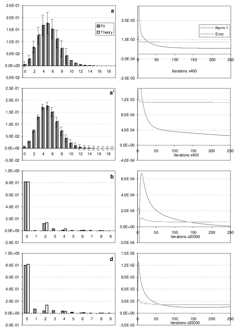
between the reconstructed distribution and the theoretical one. In Figs. 2-4 (right) we report versus the number of iterations for different signals. As it is apparent from the plots, the total error is a good marker for the convergence of the algorithm, while the normalization factor (ideally zero at each step) is not. Notice, however, that the minimum of the total error does not always coincide with the maximum fidelity of reconstruction (Figs. 6 and 7), which means that our method is slightly biased, especially for fast reconstruction, i.e. when it converges quickly as it happens for coherent signals. We have numerically observed that this problem can be circumvented by using a number of iterations approximately equal to the number of data. Currently we have no precise explanation of this phenomenon, and provide it as a heuristic prescription leading to best performances for a large class of quantum signals.

We have performed simulated experiments for coherent states , squeezed states and superposition of Fock states , where is the displacement operator and is the squeezing operator. Squeezed states have been parametrized through the total average photon number and the squeezing fraction
| (24) |
The value corresponds to a squeezed vacuum and to a coherent state. As shown in Fig. 2, the algorithm converges quite fast for coherent states, while for nonclassical states such as squeezed states (Fig. 3) the number of needed iterations is larger. The right plots in Fig. 3 also indicate that increasing does not always improve accuracy. In Fig. 4 we show reconstruction for the unbalanced superpositions of Fock states .
Concerning the values of the quantum efficiency, we used values of uniformly distributed in with and . In principle, a different distribution (not uniform) may influence the performances of the algorithm. We found, however, that both convergence and accuracy are not much affected by a different choice, which may become relevant only if the spacing between the efficiency values becomes smaller. It should be noticed that the algorithm works well also when is considerably smaller than unit. This is a relevant feature of the method in view of its experimental implementations in different working regimes. In Figs. 2-4 (bottom left) we report the reconstructions obtained assuming (coherent states and superpositions) and (squeezed states).

In experiments where we have no a priori information on the state under investigation it could happen that part, or even most, of the number distribution lies outside the reconstruction region (from to ). In this case we have checked that the algorithm is able to reconstruct accurately the norm of the included part, such that a simple check of the distribution norm allows to optimize (and in turn ) in few steps. This is a remarkable feature of the algorithm, since in general a large improves convergence but doesn’t guarantee better accuracy.


The error bars in the plots have been calculated using the Fisher information (20), that explicitly reads:
| (25) |
where is the total number of no click events.

A question may arise about the robustness of the method against fluctuations in the value of the (which, in the case of the interferometric implementation of Fig. 1, may occur as a consequence of phase fluctuations), i.e. whether or not their precise knowledge is needed. In order to check robustness we have performed simulated experiments where, during the run, the quantum efficiency may fluctuate. In particular, we assumed each uniformly distributed in the range , where
| (26) |
and is a positive number. The value corresponds to each fluctuating in an interval as large as the spacing around its expected value. The values of change accordingly during the run. Our results are summarized in Fig. 7. The reconstruction is not dramatically affected by fluctuations, though errors bars are slightly larger. We conclude that the method is robust against fluctuations.
V Conclusions
We analyzed in details an iterative algorithm to infer the photon distribution of a single-mode radiation field using only avalanche photodetectors. The method is accurate and statistically reliable for a large class of Gaussian (coherent and squeezed) and non Gaussian states (superpositions and mixtures of states), provided that on/off photodetection may be performed at different quantum efficiencies. The scheme involves only simple optical components, and allows reconstruction with APD quantum efficiency considerably smaller than unit. The convergence of the method, and its robustness against fluctuations of quantum efficiency have been demonstrated numerically, by means of Monte Carlo simulated experiments.
Acknowledgments
We thank M. Bondani and A. Ferraro for reading of the manuscript, and Z. Hradil for pointing out relevant references, and for his friendly suggestions. MGAP thanks Marco Genovese for a fruitful discussion.
References
- (1) L. Davidovich, Rev. Mod. Phys. 68, 127 (1996).
- (2) M. L. Lebedev, A. I. Filin and O. V. Misochko, Meas. Sci. Technol. 12, 736 (2001).
- (3) L. Mandel, Rev. Mod. Phys. 71, S274 (1999).
- (4) J. Kim, S. Takeuchi, Y. Yamamoto, and H.H. Hogue, Appl. Phys. Lett. 74, 902 (1999); C. Kurtsiefer, S. Mayer, P. Zarda, and H. Weinfurter, Phys. Rev. Lett. 85, 290 (2000); M. Pelton, C. Santori, J. Vukovic, B. Zhang, G.S. Solomon, J. Plant, and Y. Yamamoto, Phys. Rev. Lett. 89, 233602 (2002).
- (5) M. Munroe et al., Phys. Rev. A 52, R924 (1995)
- (6) G. M. D’Ariano, M. G. A. Paris and M. F. Sacchi, Advances in Imaging and Electron Physics 128, 205 (2003).
- (7) M. Raymer, M. Beck in Quantum states estimation, M. G .A Paris and J. Řeháček Eds., Lect. Not. Phys. 649 (Springer, Heidelberg, 2004), at press.
- (8) A.P. Dempster, N.M. Laird, D.B. Rubin, J. R. Statist. Soc. B 39, 1 (1977); Y. Vardi and D. Lee, J. R. Statist. Soc. B 55, 569 (1993).
- (9) R. A. Boyles, J. R. Statist. Soc. B 45, 47 (1983); C. F. J. Wu, The Annals of Statistics 11, 95 (1983).
- (10) D. Mogilevtsev, Opt. Comm 156, 307 (1998); Acta Phys. Slov. 49, 743 (1999).
- (11) J. ehek, Z. Hradil, O. Haderka, J. Peina, Jr., and M. Hamar, Phys. Rev. A 67, 061801(R) (2003); O. Haderka, M. Hamar, J. Peina, Eur. Phys. Journ. D 28, (2004).
- (12) K. Banaszek, Acta Phys. Slov. 48, 185 (1998); Phys. Rev A 57, 5013 (1998).
- (13) H. Cramer, Mathematical Methods of Statistics, Princeton University Press, Princeton, NJ, 1946.