Analysis of Superoscillatory Wave Functions
Matt S. Calder, Achim Kempf
Department of Applied Mathematics, University of Waterloo
200 University Avenue West, Ontario N2L 3G1, Canada
Abstract. Surprisingly, differentiable functions are able to oscillate arbitrarily faster than their highest Fourier component would suggest. The phenomenon is called superoscillation. Recently, a practical method for calculating superoscillatory functions was presented and it was shown that superoscillatory quantum mechanical wave functions should exhibit a number of counter-intuitive physical effects. Following up on this work, we here present more general methods which allow the calculation of superoscillatory wave functions with custom-designed physical properties. We give concrete examples and we prove results about the limits to superoscillatory behavior. We also give a simple and intuitive new explanation for the exponential computational cost of superoscillations.
1. Introduction
It used to be believed that a function could not oscillate much faster than its highest Fourier component. Aharonov, Berry and others showed that this is not the case by giving explicit counter-examples which they named superoscillatory functions, see, e.g., [1]-[4]. In fact, there are functions which on arbitrarily long stretches oscillate arbitrarily faster than their highest frequency Fourier component, see [5]. In other words, the presence of localized fast oscillations in a continuous function need not be visible at all in the function’s global Fourier transform. In a function’s global Fourier transform, contributions from regions of fast oscillations can be cancelled perfectly by contributions from regions where the wave function is oscillating slowly.
In the context of quantum theory, wave functions that superoscillate are able to cause a number of counter-intuitive effects. Some of these may be of conceptual significance in quantum gravity, see [6, 7]. But effects of superoscillations also enter in the low energy realm of nonrelativistic quantum mechanics. Among such potentially observable low-energy effects is the counter-intuitive phenomenon that particles with superoscillatory wave functions can be made to accelerate when passing through a neutral slit:
Consider a particle which possesses a bounded momentum range, i.e., its momentum wave function vanishes for momenta that are larger than some . As will be explained below, we can arrange that in a certain region in space the particle’s wave function superoscillates, i.e. that it oscillates with a much shorter wavelength than . Now let the wave function be incident onto a screen with a single slit in such a way that it is the superoscillatory part of the wave function which passes through the slit. Upon emerging from the slit the particle’s wave function will then oscillate rapidly where the slit is and will be zero elsewhere. The very short wavelengths of the emerging wave function will be visible in its global Fourier transform. This is because the contributions to the global Fourier transform which come from the fast oscillations in the slit interval are no longer cancelled by contributions from outside the slit interval. Therefore, the particle will have gained momentum merely by passing the slit. The momentum gain is determined by the shortness of the wave-length of the superoscillations and, as explained below, there is no limit, in principle, to how short that wavelength can be made.
In order to facilitate the design of experiments that can realize the effects of superoscillatory wave functions it is desirable to possess methods for explicitly calculating superoscillatory wave functions with predetermined properties. In particular, one may wish to calculate those low-momentum but superoscillatory wave functions which after passing through the slit yield wave functions with a predetermined arbitrarily large momentum and a momentum uncertainty that is as small as is allowed by the uncertainty relation. Our aim here is to develop methods that allow us to solve this and other problems.
Our starting point will be the method for calculating superoscillatory wave functions which was developed in [6] using results of [8] and [9]. This method allows the construction of wave functions of arbitrarily low fixed frequency content that pass through an arbitrary finite number of pre-specified points. Figures 1 and 2 show an example.
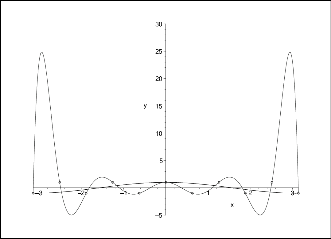
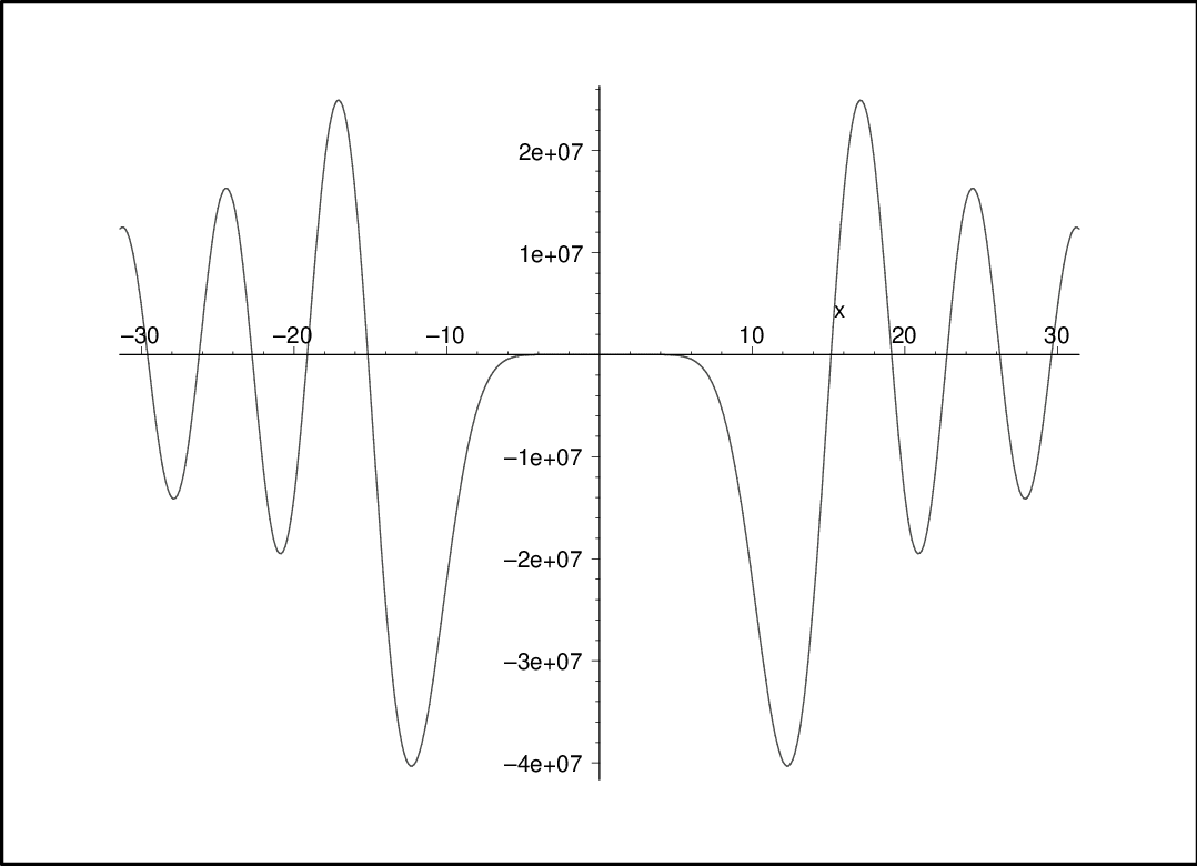
Our aim is to develop more general methods for designing superoscillatory functions with generic pre-specified properties. We will also ask what the in-principle limits are for the construction of superoscillatory wave functions.
2. Self-acceleration through single slit
In order to motivate and formalize the mathematical problem that we will address, let us consider the illustrative example of particles that self-accelerate when passing through a slit.
2.1. Notation
We will denote a wave function and its Fourier transform by the same letter, since they correspond to the same vector in the Hilbert space of states.
| (1) |
In the text, whenever necessary, we will write or to indicate if the position or the momentum wave function is meant. We will often consider particles whose momentum is bounded by a finite value :
| (2) |
Borrowing terminology from communication engineering and sampling theory, see e.g. [10], we will speak of such a function as having bandwidth , as being band-limited, or in this case as being momentum-limited. It will be convenient to define the sinc function as:
| (3) |
Notice that definitions of the sinc function elsewhere may include a factor of .
2.2. Gedanken experiment
Let us consider a particle in two dimensions which travels along the -direction towards a screen which is parallel to the -direction. Assume the particle passes through a slit with -coordinate interval in the screen. Henceforth, we will assume that the incident particle’s momentum parallel to the screen, , has a finite bound :
| (4) |
Our aim is to compare the particle’s momentum parallel to the screen before and after the particle passes the slit. For simplicity, we will suppress the variables and . From now on, is renamed and is renamed . We denote the incident wave function just before passing through the slit by and we denote the wave function which emerges from the slit by . The state is of course given by projection and renormalization
| (5) |
where projects onto the slit:
| (6) |
Similarly, we define as the projector onto a finite momentum interval:
| (7) |
While the incident wave function is momentum limited, , the emerging wave function is position limited, obeying .
As was shown in [5, 6], it is always possible to find incident wave functions which obey the momentum bound and which at any finite number of points in the slit interval take arbitrarily prescribed amplitudes (we will reproduce this result as a special case below). We will be able to arrange, therefore, that the wave function takes for example the alternating values at an arbitrarily large number of points in the slit interval - which enforces superoscillations. These will be differentiable and square integrable. Then, if the particle passes the slit, only the superoscillating stretch of the wave function emerges from the slit. Renormalized, we denote it . The Fourier transform of will show the presence of small wavelengths, implying that the particle emerges from the slit accelerated to a momentum beyond .
2.3. Template Functions
As already mentioned, the results of [5, 6] showed that functions of fixed bandwidth can always be found which at arbitrarily but finitely many points possess predetermined amplitudes. Therefore, the width or narrowness of the slit does not limit how short the wavelength of the superoscillations can be. As a consequence, there is no slit-dependent limit to the amount of self-acceleration that can be achieved in this way.
This leads us to ask more generally whether the process of self-acceleration can be designed virtually at will: is it always possible to construct incident wave functions of fixed momentum limit which on the slit interval match any arbitrarily-chosen template function, say ? This is of interest because, if true, we can optimize the predictability of the self-acceleration. To this end, we would choose the template function to be a wave function with a fixed arbitrarily large momentum expectation whose momentum uncertainty is as small as allowed by the uncertainty relation. If the incident superoscillatory wave function matched this template function in the slit interval (up to normalization), then the wave function would merge from the slit with the chosen momentum expectation and lowest possible momentum uncertainty, , for the given width of the slit. For later use, let us calculate these ideal template functions .
2.3.1. Ideal Template Functions
Our aim is to find ‘ideal’ template functions defined on the slit interval which minimize the momentum uncertainty , possess a predetermined momentum expectation and are normalized . To this end, we need to solve the constrained variational problem with the functional
| (8) |
where and are Lagrange multipliers. Note that minimizing is equivalent to minimizing because is fixed. Hence the Euler-Lagrange equation in position space is:
| (9) |
Since any wave function that emerges from the slit vanishes at the slit boundaries, we require . The solution is unique up to a phase:
| (10) |
Its uncertainties are and . We have which is a little larger than what the uncertainty relation allows because our problem requires template functions to be zero outside the slit interval.
2.3.2. Superoscillatory Wave Functions Cannot Match Arbitrary Templates
Let us now come back to the question whether it is generally possible to find an incident wavefunction which obeys a momentum bound while in the interval agreeing completely with an arbitrarily chosen template function , such as the function just calculated in Sec.2.3.1. Strictly speaking, the answer is no:
As is easily verified, all bandlimited functions are entire functions. In particular, any momentum-limited incident wave function is entire and it is, therefore, everywhere differentiable. Now choose, for example, a template function which is not differentiable at some point in the interval . Thus, there cannot exist a momentum-limited incident wave function which obeys for all . Nevertheless, a slightly weaker proposition does hold.
2.3.3. Convergence Towards Arbitrary Template Functions
Let be a continuous and square integrable template function. Let us ask whether one can always find a sequence of wave functions of fixed momentum bound which behave with more and more precision like over the region of the slit. To be precise, is it possible to find a sequence of momentum-limited incident waves whose emerging wave functions have asymptotically vanishing -distance to an arbitrary template state ? This is indeed the case.
To see this, consider in the quantum mechanical Hilbert space of states with scalar product
| (11) |
and the following three subspaces:
| (12) | ||||
| (13) | ||||
| (14) |
That is, is the subspace of states with position-limitation to the slit, is the subspace of states with fixed momentum-limitation , and is the subspace of states obtained after passing the momentum-limited wave functions through the slit.
Proposition 1.
is dense in , i.e.:
| (15) |
Proof.
If , then take . For we must show that:
| (16) |
Since is position-limited, this is equivalent to showing that:
| (17) |
Assume, for a contradiction, that:
| (18) |
This implies that . Thus, on . But, since is entire and zero over a finite interval, everywhere on , i.e., . This is a contradiction. Therefore, is dense in . ∎
While this result proves the existence of bandlimited functions that are arbitrarily close in the topology to any template function within the window of the slit, the result does not provide explicit methods for constructing such bandlimited functions.
3. Constructive Method for General Linear Constraints
We now focus on practical methods for calculating superoscillatory wave functions that approximate template functions in the slit interval. We begin with the method for constructing superoscillatory functions presented in [6]. This method allows one to specify that the to-be-found superoscillatory function takes arbitrarily chosen amplitudes at any finite number of arbitrarily chosen points :
| (19) |
The superscript (u) is to indicate that the function will generally be unnormalized. Eq.19 specifies a function which possesses a superoscillating stretch. For example, we may choose the spaced closer than and the amplitudes alternating, e.g. . The normalized wave function then possesses superoscillations that are as rapid as those of but with a renormalized amplitude. Thus, in order to obtain the with the most pronounced superoscillations, i.e. the superoscillations of largest possible amplitude, one needs to find that function whose norm is minimal. The method of [6] solves this optimization problem.
We now generalize the method of [6]. To this end, we begin by rewriting the requirement that be bandlimited by and pass through the points , namely (19), in momentum space as
| (20) |
Our aim is to obtain a method for constructing superoscillatory wave functions which not only pass through predetermined points but which obey also more generic types of constraints. To this end, let us allow constraints on the function which are of the general linear form:
| (21) |
Here, the are arbitrary linearly independent differentiable functions. By choosing these, we will be able to prescribe for the superoscillatory wave function not only amplitudes but also arbitrary derivatives, integrals and any other linear constraint. In order to obtain the most pronounced superoscillations in the normalized function we minimize the norm of , subject to the constraints in Eq.21. The to-be-optimized functional with Lagrange multipliers reads
| (22) |
leading to the Euler-Lagrange equation:
| (23) |
Recall that is zero outside the interval by assumption. Thus, using (23) in (21),
| (24) |
where the Hermitian matrix is defined by:
| (25) |
As we will show below, is invertible. Thus, , i.e.:
| (26) |
Thus, using the Fourier transform of the constraint function
| (27) |
we obtain from (23) that the desired superoscillatory (still unnormalized) incident wave function in position space is given by:
| (28) |
3.1. Existence of the Solution
It remains to be shown that is indeed invertible. To see this, let be an arbitrary vector. Then:
Since the are linearly independent the integrand is positive. Therefore, is positive definite and hence invertible.
4. The Cost of Superoscillations
As was shown in [6], one cost of superoscillations is that requiring more or faster superoscillations makes the matrix increasingly difficult to invert numerically, as its smallest and largest eigenvalues differ by growing orders of magnitude. The condition number was found to increase exponentially with the number of superoscillations.
We here only remark that, in the sense of computational complexity, this makes it computationally hard to calculate superoscillations. Interestingly, this also means that any quantum effect that naturally produces functions with arbitrarily large superoscillatory stretches constitutes an example of an exponential speed-up in the sense of quantum computing. Physical occurrences of superoscillations, e.g. in the context of evanescent waves, have been discussed e.g. in [3, 4]. Also, for example, (rather speculatively) the possibility of an unbounded production of superoscillations has been discussed in the context of the transplanckian problem of black holes in [11, 12].
Here, we will focus on a more immediate cost of superoscillations, namely the need for an increasingly large dynamical range: a function’s superoscillations are generally of low amplitude when compared to the function’s amplitudes to the left and right of its superoscillatory stretch. To be precise, it was shown in [6] that the norm of the function increases polynomially with the frequency of the prescribed superoscillations, for fixed prescribed superoscillating amplitudes. In particular, it was also shown that the norm increases exponentially with the number of imposed superoscillations. Correspondingly, in normalized wave functions the amplitudes of superoscillations decrease exponentially with the number of superoscillations. (Of course, if the superoscillating stretch of the particle’s wave function happens to pass through the slit then its wave function, however small, is re-normalized whereby the superoscillating amplitudes will be restored to the amplitudes of the template function.)
By making use of the special properties of prolate functions these scaling results were derived for the type of superoscillations produced with method of [6]. In the following two subsections we will show more directly the underlying reason for this exponential behavior of the norm of superoscillatory functions. Our argument will apply more generally to all superoscillatory functions that arise from linear constraints.
4.1. Derivatives and Norms
If a function is bandlimited one would expect that there is a bound on its derivatives. Applying the Cauchy-Schwarz inequality, consider
Thus,
| (29) |
Thus arbitrarily large derivatives, as they can be produced with superoscillations, are consistent with a finite fixed bandwidth but we see that the cost must be an increase in the norm of the function .
4.2. The Norm of Superoscillating Functions
A precise expression for the norm of the superoscillatory functions obtained by our method can be derived:
| (30) |
Hence:
| (31) |
Note that is a positive self-adjoint matrix. We now see that for given constraint functions, , the most norm-expensive superoscillatory functions are obtained if we choose the constraint parameters such that is the eigenvector of with largest eigenvalue. We will arrive at those extreme superoscillations also from independent momentum space considerations in Sec.6.
4.3. Adding Successive Constraints
Consider a set of constraints, described by a set of functions and parameters and suppose that, using our method, the momentum-limited wave function which obeys all those constraints and is of minimum norm has been calculated. Let us ask how the norm of the solution to this problem changes if we add one additional constraint
| (32) |
where and are chosen arbitrarily. Let us denote the solution to the initial problem of constraints by and let us define:
| (33) |
Clearly, if we choose the st constraint with then is also the function of minimum norm obeying the constraints, i.e. , just as if we had not added a new constraint, or as if we had set the st Lagrange multiplier to zero: .
Now, let us allow the constraint parameter to vary away from . Correspondingly, our method will yield a family of functions, , parametrized by . We observe from (31) (letting the sum run to ) that the norm squared of these functions is a quadratic (and of course positive) polynomial in . Note that its minimum occurs if we choose the -value
| (34) |
because then . Using (24) we see that this choice of leads to the vanishing of the Lagrange multiplier , which is what we expected for if we add a new constraint that is already satisfied, will not change.
Crucially, we now see that as we tune away from , say in order to enforce an additional superoscillation twist, the squared norm of the solution increases quadratically. Therefore, if we keep adding new generic constraints, say in order to implement more and more superoscillations, this will generally increase the norm of the solution by a factor in each step. Thus, the norm of the solution will generically scale exponentially with an increase in the number of constraints .
5. Applications to an ‘Ideal’ Template Function
In Sec.2.3.1, we asked how the wave function that emerges from the slit would have to look in order to describe a particle with an arbitrarily high predetermined momentum expectation value and a momentum uncertainty which is as small as is allowed by the uncertainty relation. This ‘ideal’ template function was given in (10).
Let us consider the concrete example, , , , and . If the emerging wave function can be arranged to be equal or close to this template function , this clearly exhibits the phenomenon of self-acceleration because the emerging momentum wave function would be peaked at , i.e. well outside the original bandwidth of , see Fig.3.

We had shown that exact matching, , is generally not possible, but we also saw that there always exists a sequence of incident waves so that for the emerging waves we have in the topology, which is here the only physically relevant topology. Thus, there are superoscillatory incident wave functions which achieve the prescribed self-acceleration properties to arbitrary precision. For illustration, let us explicitly calculate such superoscillatory incident wave functions.
5.1. Method of Matching Amplitudes
Let us begin by applying the method presented in [6], which is a special case of our method of general linear constraints. In this special case, we require the momentum-limited incident wave to exactly match the amplitude of the ideal template function at several points of the slit interval . The constraints in the variational problem are then given by the linearly independent constraint functions and constraint parameters . Thus,
| (35) |
which leads to the solution:
| (36) |
where and where
| (37) |
We observe that the wave function is a linear combination of sinc functions centred at the and we note that is square integrable, since the sinc functions are. In general, ill-conditioned, i.e. care must be taken to invert it with enough numerical precision so as to satisfy the constraints with sufficient accuracy.
We used routines in Maple which calculate by solving using Gaussian elimination. Concretely, we required to match the ideal template function with at equidistantly-spaced points from slit boundary to slit boundary. For example, Fig.4 shows the imaginary part of the superoscillatory function over the slit interval. Fig.5 shows a zoomed-out view of , displaying the typical big amplitudes to the left and right of the superoscillating stretch.


The momentum expectation value for the ideal template function that we chose is . Numerically, we found that the strictly momentum limited incident wave function for yields an emerging wave function whose momentum expectation value is . Clearly, the momentum of particles which pass through the slit essentially doubles by self-acceleration, as intended. The momentum uncertainty of the emerging wave function is .
Recall that for this slit size the momentum uncertainty could be significantly smaller, namely , as is precisely realized in the ideal template function. By increasing , we can achieve that the incident wave function better matches the template, leading to a lowering of towards that limiting value. For example, for we find and . For significantly larger the exponential computational expense sets in. Our generalized method for linear constraints allows us to use other linear constraints which we found to be numerically more efficient in the sense of allowing us to reach larger values of . We will discuss the use of these alternative constraints in Sec.5.2.
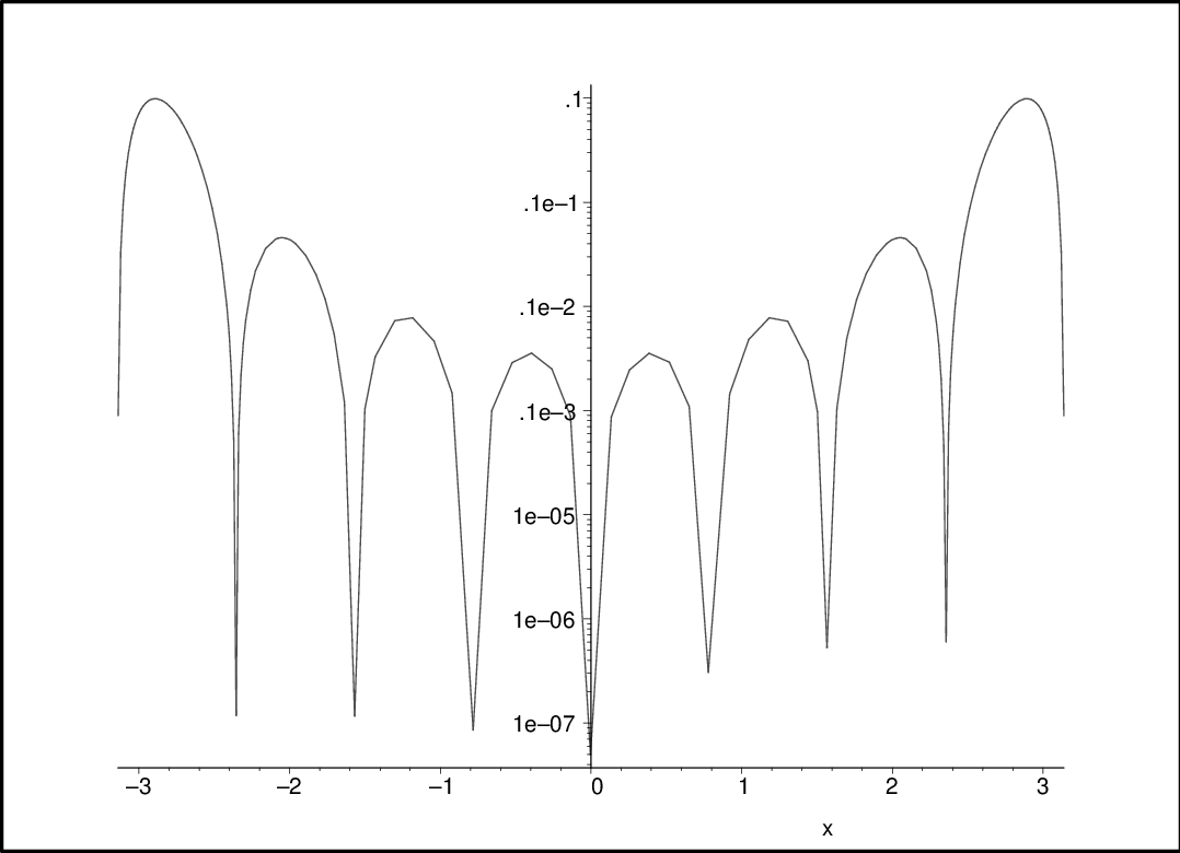
Fig.6 shows the accuracy with which the obtained by matching amplitudes of to those of agrees with the ideal template function for arbitrary in the slit interval. The behavior is similar for all values of (that we tested). For general , there are peaks and the height of the highest peak decreases with .
5.2. Method of Matching Derivatives
In order to illustrate the generality of our new method of Sec.3, let us now construct superoscillatory wave functions by requiring that the wave function matches value and derivatives of the template at one point, instead of requiring, as we did in Sec.5.1, that the wave function matches only the value of the template function at several points.
Concretely, let us require that the value and first derivatives of the to-be-found wave function agree at with those of the ‘ideal’ template function of above. In the equation for general linear constraints, (21), we obtain a constraint on the st derivative by choosing for the constraint function:
| (38) |
Matching the derivatives to those of the template is to choose the constraint parameters to be , where denotes the st derivative. Since the are linearly independent,
| (39) |
is invertible, yielding the solution
| (40) |
where
| (41) |
Note that is a linear combination of derivatives of sinc functions, each of which is bandlimited. In this case, is simpler to invert and we can go, for example, to the case before the exponential computational expense sets in. In this case, for large the coefficients quickly grow large and hence the subtle cancellations in the Fourier transform require fast increasing numerical precision.

We considered the example where the value of the function and its first 22 derivatives is required to match those of the ideal template function at . We found numerically that the momentum-limited superoscillating function, after passing through the slit, then exhibits a momentum expectation value of and momentum uncertainty . Thus we reach the targeted momentum-doubling self-acceleration, with a momentum uncertainty which is only marginally above the uncertainty relation limit for this slit size. Fig.7 displays the accuracy .
6. A Momentum Space Method
In position space, superoscillatory wave functions generally possess a characteristic shape: rapid but small oscillations in the superoscillating stretch and a few large long-wavelength amplitudes shortly before and after. Do these states also possess a characteristic shape in momentum space?
Let us consider, for example, the superoscillations obtained by prescribing oscillating amplitude values at close-by points . We found that, in momentum space, such a state is a linear combination of plane waves :
| (42) |
It appears, see e.g. Fig.8, that these generally possess small amplitudes in most of the momentum interval , except for the near the boundaries . We calculated the Fourier transforms of a number of superoscillatory wave functions and observed this as a general feature.
Thus, in momentum space, these superoscillations appear to be a linear combination of plane waves whose interference is close to being as strong as it can be, with the effect that the resulting function is of minimized norm.

If this assumption is correct, we should be able to derive superoscillatory wave functions by calculating that linear combination of plane waves in momentum space whose norm is minimal. To this end, let be points in . Our aim is to find a coefficient vector of fixed length, say such that
| (43) |
is of minimum norm. The constrained optimization problem with Lagrange multiplier
| (44) |
leads to:
| (45) |
Thus, the coefficient vector which solves this optimization problem must be eigenvector to . From Eq.30, we obtain the general expression for the norm: . Thus, must be that eigenvector of with the smallest eigenvalue.
Indeed, the position wave function determined by these coefficients is superoscillatory: already in Sec.4.2, we encountered the wave functions whose coefficient vectors are the eigenvectors of of largest eigenvalue. There, we found that these are the superoscillatory wave functions which for a given set of constraint points are most norm-expensive and which, therefore, possesses the most pronounced superoscillations.
7. Open Problems
We know from Sec.2.3.3 that it is always possible to find incident wave functions of fixed momentum bound that in the slit interval are matching any given template function arbitrarily closely in the norm topology. Thus, for all practical purposes, the self-acceleration phenomenon can be tailored at will. Our method of general linear constraints can be used to explicitly construct a sequence of momentum-limited superoscillatory wave functions which more and more closely match any given template function . The approach in the slit interval in the sense that they obey more and more linear constraints that tie to .
In Sec.5.1 and Sec.5.2 we showed that a close approach to a fixed template function can be done numerically efficiently. Clearly, intuition and the easily achieved numerical accuracy lead us to conjecture that our methods for producing superoscillations, as used in Secs.5.1,5.2, do indeed always lead to convergence in the -topology towards the template function. So far, however, we have no proof that our particular method for producing superoscillatory wave functions from linear constraints does indeed realize the convergence to generic template functions.
7.1. Quadratic constraints
Let us ask, therefore, if there is a choice of linear constraints that directly targets the area under the functions and that thereby directly guarantees convergence in the sense.
One may try, for example, constraints which require that the functions and enclose equal areas on certain subintervals of the slit. This can be put into the form of a linear constraint: Let be equidistantly-spaced points in . We require the linear constraints of (21) with the constraint functions
| (46) |
and the constraint parameters:
| (47) |
While this can easily be carried out, these constraints are not directly guaranteeing convergence towards the template function by refining the partition of the slit interval into increasingly smaller subintervals: in principle, even functions that enclose equal areas on a very small interval may have very different amplitudes. Let us, therefore, consider to impose constraints which require the area of the function on small subintervals to be small. It is clear that to this end it would be necessary to implement also constraints that are quadratic in the field . We will here not pursue this strategy to the end. As a preliminary step, however, let us generalize our method for constructing superoscillatory functions to include quadratic constraints.
To this end, we formulate the variational problem of finding the function of smallest norm and with momentum cutoff which satisfies linear and quadratic constraints that tie it to a template function :
| (48) | |||||
| (49) |
The to-be-optimized functional with Lagrange multipliers and , reads
| (50) | |||||
and the Euler-Lagrange equation reduces to
| (51) |
7.2. A Conjecture
Consider the case of a differentiable template function whose derivative is bounded: , for some finite . Assume that is a sequence of incident wave functions, calculated through the method of Sec.5.1 with the amplitudes of and matched at equidistantly-spaced points . We conjecture then that the supremum for all and all is finite as well:
| (52) |
for some finite . This is plausible because, else, would have to develop arbitrarily sharp spikes away from the template function in between some two points where its amplitudes are matched to those of the template function. From Sec.4.3, however, we expect large oscillations in the superoscillating stretch to be norm-expensive and therefore be prevented from occurring, given that the are optimized to possess minimum norm for a given set of constraints.
7.3. Convergence
Proposition 2.
Assume that the conjecture of Sec.7.2 holds true. Then, converges uniformly and in the topology over the interval to for .
Proof.
Partition the slit into equal-length intervals with the endpoints . Define by
| (53) |
That is, is the closest point in the partition from the left to . Then,
| (54) |
where we applied the triangle inequality and the mean value theorem. We therefore have uniform and -convergence. ∎
8. Summary
We started with the method for calculating superoscillatory wave functions introduced in [6] and applied it to concrete examples. We then generalized this method so that it now allows us to construct superoscillatory low-momentum wave functions with a wide range of predetermined properties. Namely, we can impose any arbitrary finite number of linear constraints. We calculated concrete examples.
Further, we addressed the question whether superoscillatory functions can be made to match any arbitrary continuous function on a finite interval. This would correspond to imposing an infinite number of constraints. Generally, the answer is no. However, we were able to prove that there always exists a sequence of superoscillatory wave functions which converges in the physically relevant topology towards any continuous template function over an arbitrarily large chosen interval.
This is of interest for example in the case of the single slit: we proved that the wave function of an incident low-momentum particle can be chosen to arbitrary precision such that, if the particle passes through the slit, it will emerge with a predetermined arbitrarily large momentum expectation and with a momentum uncertainty that is as small as permitted by the width of the slit.
Our method for constructing superoscillating wave functions allows us to construct superoscillatory wave functions which match any finite number of properties of a given template function (such as the template function’s amplitudes or derivatives at specified points). This leads to the question if by letting the number of constraints, , go to infinity we can obtain one of those sequences of superoscillatory wave functions which converge towards the template function in the topology.
We proved that such sequences exist but we have not proved that our particular method produces such sequences. The numerical evidence certainly suggests that this is the case. In fact, we found rather fast numerical convergence.
Nevertheless, it would be highly desirable to be able to prove that a given method for producing superoscillations can be used to calculate a sequence of superoscillatory functions that converges in the topology towards any given template function on an interval. An investigation based on Weierstrass’ approximation theorem is in progress, [13].
Lastly, we found a method for identifying a class of superoscillatory functions by looking at their behavior in momentum space: superoscillatory functions can be viewed as functions which in momentum space are a linear combination of plane waves with coefficients such that their interference is maximal, i.e. such that their norm is minimal.
Acknowledgement: This work has been supported by NSERC, CFI, OIT, PREA and the Canada Research Chairs Program.
References
- [1] Y. Aharonov, J. Anandan, S. Popescum, L. Vaidman. Phys. Rev. Lett. 65 2965 (1990)
- [2] Y. Aharonov, B. Reznik, A. Stern, Phys. Rev. Lett. 81 2190, (1998)
- [3] M. V. Berry, J. Phys. A27 L391 (1994)
- [4] M. Berry, Proc. Intl. Conf. on Fund. Aspects of Quantum Theory, Columbia, SC, USA, 10-12 Dec. 1992 Eds. J.S. Anandan, J. L. Safko, World Scientific, Singapore (1995)
- [5] A. Kempf, J. Math. Phys. 41 2360 (2000)
- [6] A. Kempf and P. Ferreira, quant-ph/0305148
- [7] A. Kempf, gr-qc/0310035, to appear in Phys. Rev. Lett.
- [8] L. Levi, IEEE Trans. Inform. Theory, 11, 372 (1965)
- [9] D. Slepian, Bell Sys. Tech. Journ. 57, 1371 (1978)
- [10] J.J. Benedetto, P.J.S.G. Ferreira, Modern Sampling Theory, Springer Verlag, Heidelberg (2001)
- [11] B. Reznik, Phys. Rev. D55 2152 (1997)
- [12] H. Rosu, gr-qc/9606070
- [13] A. Kempf, B.G. Bodmann, in preparation