Gates for the Kane Quantum Computer in the Presence of Dephasing
Abstract
In this paper we investigate the effect of dephasing on proposed quantum gates for the solid-state Kane quantum computing architecture. Using a simple model of the decoherence, we find that the typical error in a CNOT gate is . We also compute the fidelities of Z, X, Swap, and Controlled Z operations under a variety of dephasing rates. We show that these numerical results are comparable with the error threshold required for fault tolerant quantum computation.
I Introduction
One of the most exciting advances in physics has been the development of quantum algorithms Shor 1997; Grover 1997 which outperform their best known classical counterparts. These algorithms are described in the absence of noise, and decoherence. In experiment this will certainly not be the case. In this paper we investigate numerically how a simple model of decoherence affect gates on the Kane quantum computer Kane 1998. The Kane quantum computer is one of a number of promising silicon based quantum computer proposals Skinner et al. 2003; Ladd et al. 2002; De Sousa et al. 2003; Vrijen et al. 2000; Friesen et al. 2003.
Dephasing in systems similar to the Kane architecture has been investigated since the introduction of the spin echo technique Hahn 1950. The nuclear spin and electronic spin decoherence times of donors in is relatively long Honig 1954; Gordon and Bowers 1958; Feher and Gere 1959; Feher 1959; Honig and Stupp 1960; Faulkner 1969; Chiba and Hirai 1972; Waugh and Slichter 1988. For example, recently a time of was measured for the electronic dephasing time, Tyryshkin et al. 2003. Although dephasing times are comparatively long, if left unchecked the accumulated errors introduced by dephasing will destroy coherence in the computation.
Using quantum error correction protocols it may be possible to correct the errors caused by decoherence. Shor 1995; Steane 1996a; Calderbank and Shor 1996; Steane 1996b; Knill et al. 2001. To successfully reduce the overall error in the system, we must correct errors faster than they accumulate, in a fault-tolerant manner Shor 1996. This consideration leads to an error threshold Aharanov and Ben-Or 1997; Gottesman 1997; Preskill 1999; Knill et al. 1998. Typically such a threshold requires the probability of introducing an error in each gate to be below to as low as . For the Kane architecture the exact threshold is still under investigation Fowler 2003. In this paper we ask, if it is possible for the Kane architecture to achieve this error threshold. To do this we must know how much error is introduced by each of the gates used in the Kane quantum computing architecture.
This paper shows the results of simulations of gates on the Kane architecture in the presence of dephasing. Single qubit gates presented here are similar to those used in Nuclear Magnetic Resonance (NMR) Cory et al. 2000; Slichter 1990 for rotations of individual qubits. Voltage fluctuations on the ‘A’ gate and stochastic modeling of the system has been investigated analytically in Refs. Wellard and Hollenberg 2002; Wellard 2001. The two qubit gates presented here use non-adiabatic pulse schemes Hill and Goan 2003.
The analysis given here is a direct analogue to that of Fowler et al Fowler et al. 2003 for the adiabatic CNOT gate. The gates analyzed in this paper are simpler, faster, and potentially higher fidelity than the adiabatic gate Hill and Goan 2003. These gates do not rely on complicated pulse shapes, but simply turning on or off the voltages applied. In contrast to adiabatic gates, the timing of these gates could easily be run off a digital clock cycle. In addition, whereas the adiabatic CNOT is required to be applied up to three times to create an arbitrary two qubit gate, using non-adiabatic schemes it is possible to create an arbitrary two qubit gate directly. For example, the swap gate analyzed here would require three adiabatic CNOT gates to construct. Using non-adiabatic schemes we are able to construct it in a single pulse sequence Hill and Goan 2003, which is much faster, simpler and higher fidelity than the corresponding adiabatic scheme.
We compare each of the gates analyzed to the error threshold for fault tolerant quantum computing. We simulate the master equation for typical values of spin dephasing expected in the Kane architecture. We find that the error in the gates analyzed is less than or comparable to that required for fault tolerant quantum computation.
This paper is organized as follows. In Section II we describe the simple model of decoherence which we use and present the master equation for the system. Section III presents the results for one qubit gates, including free evolution in subsection III.1, Z rotations in subsection III.2 and X rotations in subsection III.3. Two qubit non-adiabatic gates are shown in Section IV. These include the CNOT gate in subsection IV.1, and the swap gate and controlled Z gates in subsection IV.2. Finally, conclusions are drawn in Section V.
II The Master Equation
A brief introduction to the Kane quantum computing architecture Kane 1998 is given here. The Kane architecture consists of donor atoms embedded in . The orientation of the nuclear spin of each donor represents one qubit.
When placed in a magnetic field applied in the direction, Zeeman splitting occurs. This is given by the Hamiltonian
| (1) |
where is the Pauli Z matrix, and the subscripts () indicate electronic (nuclear) spin. The magnetic field, , may be controlled externally. The application of a resonant rotating magnetic field adds the following terms to the spin Hamiltonian:
| (2) | |||||
The electronic spins couple to their corresponding nuclear spins via the hyperfine interaction,
| (3) |
where is the strength of the interaction. The design of the Kane quantum computer calls for control of the strength of the hyperfine interaction externally by applying appropriate voltages to ‘A’ gates. The electronic spins couple to adjacent electrons via the exchange interaction
| (4) |
where and are two adjacent electrons, and J is the strength of the exchange interaction which may be controlled externally through the application of voltages to the ‘J’ gates.
Altogether the spin Hamiltonian of a two donor system is given by
| (5) |
The times and fidelities of the gates naturally depend on exactly which parameters are used to calculate them. For many of the gates in this paper the typical parameters shown in Table 1 were used. These parameters are similar to the parameters used for the pure state calculations in Hill and Goan 2003.
| Description | Term | Value |
|---|---|---|
| Unperturbed Hyperfine Interaction | ||
| Hyperfine Interaction During Z Rotation | ||
| Hyperfine Interaction during X Rotation | ||
| Constant Magnetic Field Strength | ||
| Rotating Magnetic Field Strength | ||
| Hyperfine Interaction during Interaction | ||
| Exchange Interaction during Interaction |
A simple model of decoherence was used for these calculations. There are many different decoherence mechanisms, but our model only considers pure dephasing (without engergy relaxation). Whereas dephasing is certainly not the only source of decoherence, it likely to be the dominant effect on a time scale shorter than the energy relaxation (dissipation) time, . For example, Feher and Gere Feher and Gere 1959 measured for nuclear spin at a temperature of , and under similar conditions. In contrast, experimentally measured times for have been much shorter. Gordon and Bowers Gordon and Bowers 1958 measured for at in isotopically enriched . Chiba and Harai Chiba and Hirai 1972 have also measured the electronic decoherence times of , finding a rate of . For the nucleus, recent results for the nuclear spin of a nucleus show a maximum value of Ladd et al. 2003.
Recently Tyryshkin et al Tyryshkin et al. 2003 obtained an experimental measurement of at and at for a donor concentration of in isotopically pure . At millikelvin temperatures the decoherence time is likely to be even longer. Additionally these measurements were carried out in a bulk doped sample, and in our case we will be considering a specifically engineered sample. Interactions such as exchange and dipole-dipole interactions contribute to the coupling between electrons. In some experiments, such as in Ref. Tyryshkin et al. 2003, these potentially beneficial coupling have been treated as sources of decoherence, but in the operation of a quantum computer these interactions can be either be decoupled or used to generate entanglement, useful for quantum computation. Hence, it is expected that may even be longer than those reported in Tyryshkin et al. 2003. Nevertheless, we use the value of as a conservative estimate for electronic dephasing time. We expect the nuclear dephasing times to be several orders of magnitude bigger than electronic dephasing times. We choose the following parameters to be typical of the systems we are considering:
| (6) | |||||
| (7) |
The typical errors presented in the tables contained in the next three sections are evaluated at these typical dephasing times.
The simple decoherence model we consider corresponds to the master equation
| (8) |
where the dephasing terms are given by
| (9) |
Characteristic dephasing rates, and are related to the dephasing rates by the equations:
| (10) | |||
| (11) |
We define fidelity (and therefore error) in terms of the actual state after applying an operation, , and the intended state after that operation, . Due to systematic errors and decoherence these states will not necessarily be the same. When comparing against a pure state , the fidelity of an operation is defined as
| (12) |
Error is defined in terms of fidelity
| (13) |
Typically we would like to know the greatest error possible for any input state. This is a computationally difficult problem. In the results which follow, the approach taken is to calculate the fidelity for each of the computational basis states, and each of the input states which would ideally generate a Bell state. This has two main benefits. The first is that a high fidelity indicates that the gate is successfully creating or preserving entanglement. The second is that Bell states are superposition states, which are susceptible to dephasing. We also calculated the effect of each gate on the four Bell input states for the CNOT gate. For typical parameters, Bell input states give similar fidelities to those shown in this paper.
Throughout this paper we will use the states and to represent the nuclear spin up and spin down states respectively. We will use the and to represent electronic spin up and spin down states respectively.
III One Qubit Gates
III.1 Free Evolution
The spin of an isolated nucleus undergoing Larmor precession in the presence of a magnetic field, Griffiths 1995. In this case it is easy to solve the master equation with dephasing exactly. Considering only the nuclear spin, we have
| (14) |
The decoherence terms has only the single term
| (15) | |||||
| (16) |
In the rotating frame, the master equation has the solution
| (17) |
This has the effect of exponentially decaying the off diagonal terms of the density matrix, but leaves the diagonal components unchanged. For a single isolated nuclear spin, the simple model has no effect on eigenstates of (i.e., there is no relaxation process for these states). In contrast, it has a dramatic influence on superposition states whose off diagonal terms decay exponentially (i.e., dephasing). Two such states are
We can easily calculate the expectation value of the Pauli matrix, , for the state
| (18) | |||||
| (19) |
For a single nuclear spin coupled to an electronic spin via the hyperfine interaction the Hamiltonian is given by
| (20) |
We assume that electron is initially polarized by the large magnetic field, . The evolution of this Hamiltonian was calculated for their typical values [given in Eq. (6), Eq. (7) and Table 1]. The fidelity after different times is shown in Fig. 1. This figure shows the Bloch sphere radius, given by
| (21) |
A pure state has a radius of one, and a radius of less than one indicates a mixed state. An initial state of was used. The radius decays at a rate governed by the nuclear decoherence time, which in this case is . As is expected, this decay is the same as the well known solution to the Bloch equations.

III.2 Z Rotations
Z rotations on the Kane architecture may be performed by varying the Larmor precession frequency of a single qubit Hill and Goan 2003. Graphs showing the error in the Z gate at different dephasing rates are shown in Figs. 2 and 3.
Figure 2 shows the error at different rates of decoherence for both electrons, , and nuclei, , for a single qubit in the state. The calculated error does not significantly depend on the electronic or nuclear dephasing rate. The pure state is not affected by decoherence terms in the master equation. Therefore the only effect of dephasing occurs when the hyperfine interaction rotates this state. The effect of dephasing on this state is negligible.
The error in the Z operation for an initial state of , is primarily due to systematic error of . This error is due to the hyperfine interaction coupling between electrons and nuclei. This allows a small probability of finding the electrons in an excited state. At typical rates of decoherence for the short duration of a Z rotation (approximately ), systematic error is the dominant effect. For the state, the typical error is .
In the previous section we noted that superposition states, and , are affected by dephasing terms more than eigenstates of . This is illustrated in Fig. 3. Electronic dephasing times have little effect on the overall fidelity. As the nuclear dephasing rate increases, the fidelity decreases, with a maximum error of approximately . This indicates all quantum coherence was lost and we are in classical mixture of the states and . For typical rates of dephasing [given in Eq. (6), and Eq. (7)], the error is found to be which is largely due to systematic error.
The maximum error, for typical rates of dephasing, of any of the states tested for the Z gate is . This error is largely due to systematic effects rather than dephasing. This error suggests it is theoretically possible to do a Z rotation with an error of less than the limit suggested for fault tolerant quantum computing. The results for the Z gate are summarized in Table 2.
| State | Systematic Error | Typical Error |
|---|---|---|
| Maximum |


III.3 X Rotations
X rotations are performed using a resonant magnetic field, . The error in the X rotation was found at different rates of dephasing. This is shown for the two basis states in Figs. 4 and 5. Evident on both of these graphs is a valley which levels out at a minimum error. This error is primarily due to systematic error in the gate. For the initial state the systematic error is found to be , and for the initial state the systematic error is found to be . As the nuclear dephasing rates, , increases, the fidelity of the operation decreases. The fidelity of the operation drops to indicating that, in the limit of large dephasing rates, the rotating magnetic field does not have the desired effect of a resonant magnetic field.
In Figs. 4 and 5, we see that the fidelity of the X rotation depends weakly on the electronic dephasing rate, . The solutions to the equations under these conditions show that the principal cause of error is the electron becoming excited to a higher energy level.
Under typical conditions, the initial state has an error of . The state has an error of . In this operation dephasing has a much more important role than in Z rotations. One reason for this is that an X rotation takes longer, approximately .
The error in the X gate is summarized in Table 3. The maximum error from the two basis states tested for the X gate was . The error induced in this operation is less than a threshold of required for fault tolerant quantum computing.
| State | Systematic Error | Typical Error |
|---|---|---|
| Maximum |


IV Two Qubit Gates
IV.1 The CNOT Gate
The CNOT gate is specified by
| (22) |
which may be created using the steps specified in Ref. Hill and Goan 2003. In the following discussion of two qubit gates, if not explicitly stated, all initial electron spin states are assumed to be .
The error in the CNOT in the presence of dephasing was found by numerically solving the master equation [Eqs. (8) and (9)] for the appropriate pulse sequence Hill and Goan 2003. For different rates of dephasing, different fidelities are obtained. Fidelities were calculated for each of the four computational basis states, and for the evolution leading to the four Bell states. Fidelities for the four computational basis states are shown in Fig. 6.


Each of the states shows a minimum error when the rates of electronic and nuclear dephasing are slow. The remaining error is due to systematic error in the gate. Some sources of systematic error for the CNOT operation include off-resonant effects, excitation into higher electronic energy levels, and imperfections in the pulse sequences (such as the break-down of the second order approximations used to derive appropriate times for pulse sequence Hill and Goan 2003). Systematic error for each of the states , , and are , , , and respectively. For evolution starting in an initial Bell state, we find the systematc error is , , and . Sytematic error for states resulting in a Bell state are shown in Table 4.
In each of the four states, as the dephasing rate increases, the fidelity decreases. In the limit of large dephasing rates, the computational basis states tend to stay in their original states. This is particularly evident from the graphs of and which have higher fidelity (lower error) at high dephasing rates. In contrast, the states and have lower fidelities (highter error) at high rates of dephasing. For example, the state stays in the state after the CNOT operation. At such high rates of dephasing, not even the single qubit rotations described in Section III.3 apply, which form part of the CNOT gate operation. For these states quantum coherence has been lost. When we consider, for example, the state we find that at a high dephasing rate of that the error of the gate is . In this case, quantum coherence has been lost between the two states, and the qubit evolves to a completely mixed state.
Electronic dephasing rates play a much bigger role in two qubit gates than in single qubit gates.
For the typical dephasing times, and [given in Eq. (6), Eq. (7)], we find the error for the states , , and are , , , and respectively. The error for an initial state of one of the four Bell states is found to be , , , and . Typical errors for states resulting in a Bell state are shown in Table 4. This implies that under our very simple decoherence model, the maximum error in the CNOT gate in any basis state is . This is only marginally under the threshold of required for fault tolerant quantum computation.
Errors for each of the computational basis states are shown in Table 4, and the maximum error of any of the four computational basis states or states with evolution leading to a Bell state is plotted in Fig. 7.
| State | Systematic Error | Typical Error |
|---|---|---|
| Maximum |

These results are directly analogous to calculations made for the adiabatic CNOT gate Fowler et al. 2003. We have used the same noise model as was used in their numerical simulations. In calculations for the adiabatic CNOT gate at decoherence times, for electronic and nuclear dephasing rates of and respectively, the maximum error of any of the four basis states for the adiabatic CNOT gate was found to be ‘just over ’ Fowler et al. 2003. In comparison, for the same conditions, we find that the maximum error in the non-adiabatic gate is . Under these conditions both non-adiabatic and adiabatic gates give similar fidelities.
Where does this error come from at the dephasing rate specified above, for the nonadiabatic CNOT gate? The error in an X rotation under these conditions is and the error in the entangling operation of the gate , is and therefore it is clear that the two qubit entangling operation is the major source of error. When electronic decoherence times are short, any electron mediated operations will be affected by this decoherence. By increasing the exchange interaction strength, the time required for the electron mediated operation may be reduced. For example, at a strength of the error decreases to and the maximum error in the CNOT gate is also for any of the computational basis states.
The advantage of nonadiabatic gates over adiabatic gates is that the pulse schemes required are much simpler, faster, and as at the conditions considered in Ref. Fowler et al. 2003, the two schemes have approximately the same fidelity. Considering the electronic decoherence times measured in Ref. Tyryshkin et al. 2003 it is likely that electronic dephasing rates are not as large as considered in Ref. Fowler et al. 2003. At lower rates of dephasing, we approach the systematic error, which may be smaller for nonadiabatic gates than adiabatic gates Hill and Goan 2003. Another distinct advantage of the nonadiabatic gates is that any two qubit gate may be made. This allows us to construct two qubit gates directly (such as the swap gate), which are faster and higher fidelity than expressing them as combinations of CNOT gates and single qubit rotations. If the Kane computer was being run from a digital clock cycle, non-adiabatic two qubit gates could be controlled at discrete times, and do not require the continuous and sophisticated pulse shapes required for adiabatic gates operating at this speed and fidelity.
IV.2 The Swap Gate and Controlled Z Gate
Similar calculations to those calculated for the CNOT gate were carried out for the swap gate and the controlled Z gate. The swap gate is specified by the matrix
| (23) |
The controlled Z gate is specified by the matrix
| (24) |
The circuit which may be used to create the swap gate may be found in Ref. Hill and Goan 2003.
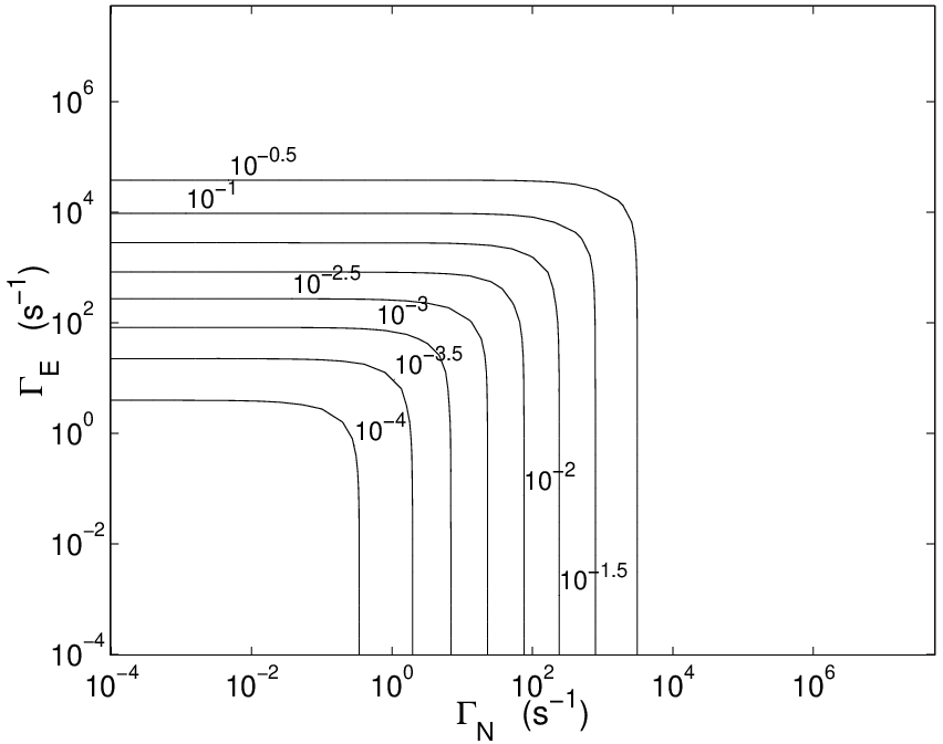
The master equation was solved numerically for each pulse sequence. The error in the swap gate was calculated for each basis state, and each state whose output state is a Bell state. Note that for these two gates the states which give Bell states as output are themselves Bell states. A separate simulation was completed for each combination of nuclear and electronic dephasing times. The maximum error of any of the basis states has been plotted in Fig. 8 for the swap gate, and Fig. 9 for the control Z gate.
Similar features that were evident for the CNOT gate are visible in these figures. The corresponding errors are shown in Table 5 for the swap gate, and Table 6 for the control Z gate.
| State | Systematic Error | Typical Error |
|---|---|---|
| Maximum |
| State | Systematic Error | Typical Error |
|---|---|---|
| Maximum |

V Conclusion
In conclusion, we have investigated the effect of dephasing on the Kane quantum computing architecture. We used a simple model of decoherence and investigated how this model affected proposed gate schemes on the Kane quantum computer. For typical decoherence rates [given in Eq. (6), Eq. (7)], these results are summarized in Table 7.
Each of the errors, for typical rates of dephasing, found here are close to the error threshold required for fault tolerant quantum computation. If the temperature is lowered, and coupling between qubits is not considered a decoherence process as in Ref. Tyryshkin et al. 2003, it is likely that the typical decoherence times for the Kane architecture may be further reduced, and therefore unambiguously under the threshold required for fault tolerant quantum computation.
Construction and operation of the Kane quantum computer is extremely challenging. In the actual physical system there will undoubtedly be noise and decoherence processes not considered in our simple physical model. This substantial effort would never be able to achieve its ultimate goal of a working quantum computer if there were fundamental reasons why such a computer could not operate. In this paper we investigated the one such effect on proposed gates for the Kane quantum computer. Our simulations indicate that errors due to dephasing, the dominant form of decoherence in the Kane architecture, do not rule out fault tolerant quantum computation.
| Gate | Typical Error | Systematic Error | Time |
|---|---|---|---|
| Z | |||
| X | |||
| CNOT | |||
| Swap | |||
Acknowledgements.
The authors would like to thank G. J. Milburn for support. This work was supported by the Australian Research Council, the Australian government and by the US National Security Agency (NSA), Advanced Research and Development Activity (ARDA) and the Army Research Office (ARO) under contract number DAAD19-01-1-0653. H.-S.G. would like to acknowledge financial support from Hewlett-Packard.References
- Shor (1997) P. W. Shor, SIAM Journal of Computing 26, 1484 (1997).
- Grover (1997) L. K. Grover, Phys. Rev. Lett. 79, 325 (1997).
- Kane (1998) B. E. Kane, Nature 393, 133 (1998).
- Skinner et al. (2003) A. J. Skinner, M. E. Davenport, and B. E. Kane, Phys. Rev. Lett. 90, 087901 (2003).
- Ladd et al. (2002) T. D. Ladd, J. R. Goldman, F. Yamaguchi, Y. Yamamoto, E. Abe, and K. M. Itoh, Phys. Rev. Lett. 89, 017901 (2002).
- De Sousa et al. (2003) R. De Sousa, J. D. Delgado, and S. Das Sarma (2003), eprint cond-mat/0311403.
- Vrijen et al. (2000) R. Vrijen, E. Yablonovitch, K. Wang, H. W. Jiang, A. Baladin, V. Roychowdhury, T. Mor, and D. DiVincenzo, Phys. Rev. A 62, 012306 (2000).
- Friesen et al. (2003) M. Friesen, P. Rugheimer, D. E. Savage, M. G. Lagally, D. W. Van der Weide, R. Joynt, and M. A. Eriksson, Phys. Rev. B 67, 121301 (2003).
- Hahn (1950) E. L. Hahn, Phys. Rev. 80, 580 (1950).
- Honig (1954) A. Honig, Phys. Rev. 96, 254 (1954).
- Gordon and Bowers (1958) J. P. Gordon and K. D. Bowers, Phys. Rev. Lett. 1, 368 (1958).
- Feher and Gere (1959) G. Feher and E. A. Gere, Phys. Rev. 114, 1245 (1959).
- Feher (1959) G. Feher, Phys. Rev. 114, 1219 (1959).
- Honig and Stupp (1960) A. Honig and E. Stupp, Phys. Rev. 117, 69 (1960).
- Faulkner (1969) R. A. Faulkner, Phys. Rev. 184, 713 (1969).
- Chiba and Hirai (1972) M. Chiba and A. Hirai, J. Phys. Soc. Japan 33, 730 (1972).
- Waugh and Slichter (1988) J. S. Waugh and C. P. Slichter, Phys. Rev. B 37, 4337 (1988).
- Tyryshkin et al. (2003) A. M. Tyryshkin, S. A. Lyon, A. V. Astashkin, and A. M. Raitsimring, Phys. Rev. B 68, 193207 (2003).
- Shor (1995) P. Shor, Phys. Rev. A. 52, 2493 (1995).
- Steane (1996a) A. M. Steane, Phys. Rev. Lett. 77, 793 (1996a).
- Calderbank and Shor (1996) A. R. Calderbank and P. Shor, Phys. Rev. A 54, 1098 (1996).
- Steane (1996b) A. M. Steane, Proc. Roy. Soc. Lond. A 452, 2251 (1996b).
- Knill et al. (2001) E. Knill, R. Laflamme, R. Martinez, and C. Negrevergne, Phys. Rev. Lett. 86, 5811 (2001).
- Shor (1996) P. W. Shor, in Proceedings of the 37th Annual Symposium on Fundamentals of Computer Science (1996), pp. 56–65.
- Aharanov and Ben-Or (1997) D. Aharanov and M. Ben-Or, in Proceedings of the Twenty-Ninth Annual ACM Symposium on the Theory of Computing (1997), pp. 176–188.
- Gottesman (1997) D. Gottesman, Ph.D. thesis, California Institute of Technology (1997).
- Preskill (1999) J. Preskill, in Introduction to Quantum Computation and Information, edited by H.-K. Lo, T. Spiller, and S. Popescu (World Scientific, Singapore, 1999), chap. Fault Tolerant Quantum Information, pp. 213–269.
- Knill et al. (1998) E. Knill, R. Laflamme, and W. H. Zureck, Science 279, 342 (1998).
- Fowler (2003) A. G. Fowler, Private communication (2003).
- Cory et al. (2000) D. G. Cory, R. Laflamme, E. Knill, L. Viola, T. F. Havel, N. Boulant, G. Boutis, E. Fortunato, S. Lloyd, R. Martinez, et al., Fortschritte der Physik 48, 875 (2000).
- Slichter (1990) C. P. Slichter, Principles of Magnetic Resonance (Springer-Verlag, Berlin, 1990), 3rd ed.
- Wellard and Hollenberg (2002) C. J. Wellard and L. C. L. Hollenberg, J. Phys. D: Appl. Phys. 35, 2499 (2002).
- Wellard (2001) C. J. Wellard, Ph.D. thesis, Unversity of Melbourne (2001).
- Hill and Goan (2003) C. D. Hill and H.-S. Goan, Phys. Rev. A 68, 012321 (2003).
- Fowler et al. (2003) A. G. Fowler, C. J. Wellard, and L. C. L. Hollenberg, Phys. Rev. A 67, 012301 (2003).
- Ladd et al. (2003) T. D. Ladd, D. Maryenko, E. Abe, K. M. Itoh, and Y. Yamamoto (2003), eprint quant-ph/0309164.
- Griffiths (1995) D. J. Griffiths, Introduction to Quantum Mechanics (Prentice Hall Inc., 1995).