Efficient quantum computation
within a disordered Heisenberg spin-chain

Many possible physical implementations for performing quantum computation have been proposed (see Ch.8 in [1] for example). However the vast majority of these schemes require that the coupling between qubits (e.g. two-level atoms or quantum dots) can be turned on and off. In addition to the difficulty of doing this sufficiently quickly so as to avoid decoherence, and sufficiently accurately so as not to introduce unwanted errors, there is the fundamental problem that coupling terms in the Hamiltonian of multi-qubit systems are permanently ‘on’, i.e. they are time-independent. Building upon the work of Refs. [2, 3], Benjamin and Bose [4] recently made a significant advance beyond this paradigm by introducing a simple method for performing quantum computation with a Heisenberg spin-chain where the spin-spin couplings are ‘always on’, i.e. constant in time. This scheme is clearly of great potential use – however, a quantitative study of its efficiency and possible generalization has not yet been reported. Futhermore the couplings between each spin-spin pair were assumed to be identical [4, 5, 6] – however, this situation cannot be engineered reliably in systems such as nanostructure arrays.

In this paper, we generalize Benjamin and Bose’s scheme to a Heisenberg spin chain with non-identical couplings between spins (i.e. qubits). Our scheme of time-independent, non-identical qubit-qubit couplings, will arise naturally in nanofabricated systems such as arrays of quantum dots, or chains of C₆₀ buckyball cages. It can also be engineered to arise for atoms in optical traps. Within a simple chain setup, we show that an arbitrary two-qubit gate can be implemented reliably with at most three relaxations of one controlled qubit. Such two-qubit gates are a crucial ingredient for universal quantum computation. This number of relaxations amounts to switching the on-site energies at most twenty-one times. The major difficulty within this type of quantum computing scheme arises when the controlled qubits are relaxed. However, our work shows that the number of times the controlled qubits are relaxed can be minimized using a simple searching procedure. Our findings should provide considerable comfort for experimentalists preparing to build candidate quantum computer systems using coupled nanostructures: Time, effort and resources do not have to be wasted on engineering identical qubit-qubit couplings.

The Hamiltonian we consider is the following:

$$H=\sum_{j}E_{j}(t)\sigma^{Z}_{j}+\sum_{j}J_{j,j+1}\underline{\sigma}_{j}\cdot\underline{\sigma}_{j+1}$$

(1)

where $j$ labels the qubit (e.g. quantum dot, C₆₀ buckyball or atom) and the qubit-qubit couplings are represented by $\{J_{j,j+1}\}$. For simplicity we consider the case where the $J$’s in each pair $(J_{j-1,j},J_{j,j+1})$ do not differ by more than ten percent in magnitude – however there is no indication that similar results will not hold outside this range. Recall that single-qubit operations can be implemented if the following sum of terms

$$\sum_{j}\left[F_{j}(t)\sigma^{X}_{j}+G_{j}(t)\sigma^{Y}_{j}\right]$$

(2)

is added to the above Hamiltonian. It is assumed that the experimentalist has control over the temporal form of the on-site energies $\{E_{j}(t),F_{j}(t),G_{j}(t)\}$. For example, these terms can be controlled by applying a magnetic field (hence changing the Zeeman energy) or electric field (hence introducing a Stark shift) to the qubit $j$ [7] in the appropriate direction. We will henceforth assume that single-qubit operations are possible (which is essentially the same assumption as adopted in Refs. [3, 4]) and will concentrate on two-qubit operations. Hence we will discard the single qubit terms given in Equation 2, since they are not needed for the discussion of two-qubit operations.

Consider three arbitrary qubits within this chain. We assume that qubits 1 and 3 are work qubits and that the qubits 0 and 4 adjacent to them are fixed. Without loss of generality, we can incorporate these interactions into the on-site energy terms of qubits 1 and 3. Focusing on qubits 1 to 3, we note that the four subspaces spanned by $\{|000\rangle\}$, $\{|001\rangle,|010\rangle,|100\rangle\}$, $\{|110\rangle,|101\rangle,|011\rangle\}$ and $\{|111\rangle\}$ are invariant under $H$. Within the basis $\{|001\rangle,|010\rangle,|100\rangle\}$, the operation $H$ is:

$$U\equiv\left(\begin{array}[]{ccc}A_{1}&2J_{23}&0\\ 2J_{23}&A_{2}&2J_{12}\\ 0&2J_{12}&A_{3}\end{array}\right)$$

(3)

where

	$\displaystyle A_{1}$	$\displaystyle=$	$\displaystyle E_{1}+E_{2}-E_{3}+J_{12}-J_{23}$		(4)
	$\displaystyle A_{2}$	$\displaystyle=$	$\displaystyle E_{1}-E_{2}+E_{3}-J_{12}-J_{23}$		(5)
	$\displaystyle A_{3}$	$\displaystyle=$	$\displaystyle-E_{1}+E_{2}+E_{3}-J_{12}+J_{23}\ \ \ .$		(6)

Within the basis $\{|110\rangle,|101\rangle,|011\rangle\}$, the operation $H$ is:

$$V\equiv\left(\begin{array}[]{ccc}B_{1}&2J_{23}&0\\ 2J_{23}&B_{2}&2J_{12}\\ 0&2J_{12}&B_{3}\end{array}\right)$$

(7)

where

	$\displaystyle B_{1}$	$\displaystyle=$	$\displaystyle-E_{1}-E_{2}+E_{3}+J_{12}-J_{23}$		(8)
	$\displaystyle B_{2}$	$\displaystyle=$	$\displaystyle-E_{1}+E_{2}-E_{3}-J_{12}-J_{23}$		(9)
	$\displaystyle B_{3}$	$\displaystyle=$	$\displaystyle E_{1}-E_{2}-E_{3}-J_{12}+J_{23}\ \ \ .$		(10)

We assume that qubit 2 is initialized to $|0\rangle$. To perform a two-qubit operation on qubits 1 and 3, qubit 2 has to be decoupled from them after the operation. Namely, $[e^{-iU\tau}]_{12},[e^{-iU\tau}]_{21},[e^{-iU\tau}]_{23}$ and $[e^{-iU\tau}]_{31}$ are all zero, where $\tau$ is the duration of the operation and $[e^{-iU\tau}]_{ij}$ denotes the $(i,j)$-entry of $e^{-iU\tau}$ in matrix form. The same requirements apply to the matrix $[e^{-iV\tau}]$. Due to unitarity of the operation, this amounts to requiring that the magnitudes of $[e^{-iU\tau}]_{22}$ and $[e^{-iV\tau}]_{22}$ equal one. If this is achieved, then the corresponding two-qubit operation will be:

$$N\equiv\left(\begin{array}[]{cccc}\alpha&0&0&0\\ 0&[e^{-iU\tau}]_{11}&[e^{-iU\tau}]_{13}&0\\ 0&[e^{-iU\tau}]_{31}&[e^{-iU\tau}]_{33}&0\\ 0&0&0&\beta\end{array}\right)$$

(11)

where

	$\displaystyle\alpha$	$\displaystyle=$	$\displaystyle e^{-i(E_{1}+E_{2}-E_{3}+J_{12}+J_{23})\tau}$		(12)
	$\displaystyle\beta$	$\displaystyle=$	$\displaystyle[e^{-iV\tau}]_{22}\ .$		(13)

Our aim now is to deduce a set of $(\{E_{j}\},\tau)$ values which will allow us to decouple the controlled qubit after time evolution $\tau$. Namely, we are searching for solutions that satisfy the two constraints: $[e^{-iU\tau}]_{22}=1$ and $[e^{-iV\tau}]_{22}=1$, in a four dimensional space. The use of various optimization techniques in gate-building in the classical domain has been explored in Ref. [8]. Here, we employ the gradient descent method with random initial positions, which is common to all control optimization problems (see Ch. 9 in Ref. [9] for example). Our search algorithm goes as follows:

1. 1.

   Given a range $L$ and density parameter $m$, we divide the set $\{E_{j}\}$ into $m$ values $\{-L+\frac{2Lk}{m-1}:0\leq k\leq m-1\}$ and we divide $\tau$ into $m$ values $\{L+\frac{3Lk}{m-1}:0\leq k\leq m-1\}$.

2. 2.

   For each of the $m^{4}$ point combinations, we calculate the corresponding matrices $U$ and $V$. These constitute the initial position of our gradient descent method to find the parameters $(\{E_{j}\},\tau)$, with objective function:

   $${\rm Obj}(\{E_{j}\},\tau)\equiv\left|[e^{-iU\tau}]_{22}\right|^{2}+\left|[e^{-iV\tau}]_{22}\right|^{2}.$$

   (14)

   We then proceed with the gradient descent method. Specifically, we first fix $\tau$ and perform a descent with respect to $\{E_{j}\}$, then we fix the set $\{E_{j}\}$ and perform a descent on the coordinate $\tau$. We repeat the process until a local minimum is attained – specifically, we repeat the process until the change in the ojective function is less than 0.000005. If the value of the objective function at that local minimum is higher than $1.99995$, we form the matrix $N$ as defined above and calculate its classifying angles as in Refs. [10, 11].

3. 3.

   If the angle is of the form $(0,0,c)$ with uncertainty $\pm 0.0025\pi$, it is recorded.

Step 1 partitions the search problem into many possible starting positions, in order that different two-qubit operations can be generated. The search in Step 2 ensures that the combination $(\{E_{j}\},\tau)$ decouples the controlled qubit from the work qubits as much as possible. We note that we separate the descents with respect to the set $\{E_{j}\}$ and to the coordinate $\tau$ because their effects on the objective function are very different. The set $\{E_{j}\}$ affects the eigenvalues and eigenvectors of the matrices $U$ and $V$ while $\tau$ acts as a scalar multiplier of the eigenvalues. The results are shown in Figure 1 with $L=5$ and $m=30$. For the coupling constants $(J_{12},J_{23})\in\{(1,0.9),(1,0.95),(1,1.05),(1,1.1)\}$, we find that almost all values of the rotation angle in the interval $[0,\pi/2]$ become represented. The largest gap between two nearest-neighbor points in terms of the rotation angle is $\sim 0.0045\pi$, while the mean gap between two nearest neighboring points in terms of the rotation angle is less than $0.0005\pi$. It takes about 8 hours of computing time for each $J$ value on a standard laptop computer. Since the algorithm is highly parallel, the computing time will be cut by one half if two computers are on and so forth. The particular coupling constants shown in Figure 1 are chosen to illustrate the algorithm – further simulations indicate that similar results should hold for other sets of values. In short, our simulations demonstrate that by controlling the on-site energies in a Heisenberg spin-chain, one can generate two-qubit gates of the form $e^{ci\sigma_{z}^{1}\sigma_{z}^{2}}$ with arbitrary $c$ with some tolerable errors. Specifically, our simulations suggest the following conjecture:

Conjecture. For all non-zero $J_{12}$ and $J_{23}$, for any $c\in[0,\pi/2]$ and for all $\epsilon>0$, there exists a set $(\{E_{j}\},\tau)$ such that

$$\left|{\rm Tr}_{2}e^{-iH(\{E_{j}\})\tau}-e^{ci\sigma^{Z}\otimes\sigma^{Z}}\right|<\epsilon$$

(15)

where Tr${}_{2}(.)$ denotes the operation of tracing out the second qubit, $H(\{E_{j}\})$ is as shown in Equation 1, and $|M|$ returns the absolute value of the entry with the maximum norm in the matrix $M$.

We have not been able to formally prove or disprove this conjecture. However we recall that our algorithm corresponds to searching for four-dimensional vectors $(\{E_{j}\},\tau)$ which satisfy two constraints: $[e^{-iU\tau}]_{22}=[e^{-iV\tau}]_{22}=1$. Hence we speculate that this excess in degrees of freedom will enable us to perform different two-qubit operations.

References [10, 11, 12] showed that an arbitrary entangling gate $Q$ can be written as $Q=S_{l}AS_{r}$, where

$$A=e^{c_{1}i\sigma^{X}_{1}\sigma^{X}_{2}}\ e^{c_{2}i\sigma^{Y}_{1}\sigma^{Y}_{2}}\ e^{c_{3}i\sigma^{Z}_{1}\sigma^{Z}_{2}}$$

(16)

with $S_{l},S_{r}\in{\rm SU(2)}\otimes{\rm SU(2)}$. Since

$$R_{k}e^{ci\sigma^{k}_{1}\sigma^{k}_{2}}R_{k}^{\dagger}=e^{ci\sigma^{Z}_{1}\sigma^{Z}_{2}}$$

(17)

where $R_{k}=e^{(\pi/4)i\sigma^{k}}\otimes e^{(\pi/4)i\sigma^{k}}\in{\rm SU(2)}\otimes{\rm SU(2)}$ and $k\in\{X,Y\}$, we see that an arbitrary two-qubit gate can be implemented by letting the controlled qubits relax three times at most. This amounts to switching the on-site energy terms twenty-one times at most. For example, since the CNOT can be represented as $(0,0,\pi/4)$ [11], it can be implemented in the present scheme with just one relaxation of the controlled qubit. We note that our measure of efficiency relates directly to the difficulties arising in physical implementations, i.e. the difficulties in relaxing the controlled qubits. Hence, the fewer number of times the controlled qubit need to be relaxed, the more efficient the computing scheme is. On the other hand, since non-trivial entangling only occurs when the controlled qubit is relaxed, one can easily relate our measure of efficiency to the number of entangling operations needed, which is the usual measure of efficiency in quantum computing (see Refs. [12, 13] for example). In this regard, our method compares well with the most recent result obtained in Ref. [13] since our results also indicate an upper bound of three relaxations/entangling operations to implement an arbitrary two-qubit gate.

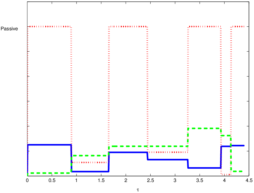
Figure 2 shows a systematic plot of the switching profiles which illustrate this result. We note that the error in decoupling qubit 2 from qubit 1 and 3 could be further reduced by running longer simulations, as shown in Figure 3. The error in coverage of the angle range can also be improved with more simulation. Its presence can also be seen as making the quantum computation more probabilistic and hence should not be viewed as being detrimental.

In conclusion, we have provided a generalization of the quantum computing scheme introduced in Ref. [4] and have also discussed its efficiency. We have found the important practical and theoretical result that identical qubit-qubit couplings are not necessary for universal quantum computation, thereby eliminating a fierce requirement on the precision of nanofabrication. We believe that the results of this work are relevant to a range of quantum computing implementations, and should stimulate experimentalists to explore less mature fabrication technologies. In particular, the flexibility of the objective function in the gradient descent step should allow experimentalists to weigh parameters differently in order to reflect particular experimental conditions, or characteristics of fabrication. For example if the length of time for temporal evolution is a major constraint, perhaps because of decoherence processes, a penalty term of the form $-\tau$ could be added to the objective function in order to skew the optimization.

In more general terms, the method introduced here is not restricted to the Heisenberg interaction Hamiltonian. Specifically, given a set of fixed parameters and a set of controllable parameters which would be determined by physical requirements, one could search over the controllable parameters to try to come up with specific gates, as in the present paper. Therefore we envisage usefulness for this scheme when applied to more general Hamiltonian systems.

References

- [1] M. A. Nielsen and I. L. Chuang, Quantum Computation and Quantum Information (Cambridge Unviersity Press, Cambridge, 2000).
- [2] D.P. DiVincenzo et al., Nature 408, 339 (2000).
- [3] X. Zhou et al., Phys. Rev. Lett. 89, 197903 (2002).
- [4] S. C. Benjamin and S. Bose, Phys. Rev. Lett. 90, 247901 (2003); quant-ph/0401071.
- [5] S. C. Benjamin, quant-ph/0403077.
- [6] A. Bririd and S. C. Benjamin, quant-ph/0308113.
- [7] D. Loss and D. P. DiVincenzo, Phys. Rev. A 57, 120 (1998).
- [8] D. H. Wolpert, J. Lawson and M. Millonas (private communication).
- [9] S. Boyd and L. Vandenberghe, Convex Optimization (Cambridge Unviersity Press, Cambridge, 2004).
- [10] B. Kraus and J. I. Cirac, Phys. Rev. A 63, 062309 (2001).
- [11] J. Zhang et al., Phys. Rev. A 67, 042313 (2003).
- [12] J. Zhang et al., Phys. Rev. Lett. 91, 027903 (2003).
- [13] G. Vidal and C. M. Dawson, Phys. Rev. A 69, 010301(R) (2004).