NMR Techniques for Quantum Control and Computation
Abstract
Fifty years of developments in nuclear magnetic resonance (NMR) have resulted in an unrivaled degree of control of the dynamics of coupled two-level quantum systems. This coherent control of nuclear spin dynamics has recently been taken to a new level, motivated by the interest in quantum information processing. NMR has been the workhorse for the experimental implementation of quantum protocols, allowing exquisite control of systems up to seven qubits in size. Here, we survey and summarize a broad variety of pulse control and tomographic techniques which have been developed for and used in NMR quantum computation. Many of these will be useful in other quantum systems now being considered for implementation of quantum information processing tasks.
I Introduction
Precise and complete control of multiple coupled quantum systems is expected to lead to profound insights in physics as well as to novel applications, such as quantum computation Bennett00a; Nielsen00b; Galindo02a. Such coherent control is a major goal in atomic physics Leibfried03a; Wieman99a; Science02a, quantum optics Zeilinger99a; Science02a and condensed matter research Makhlin01a; Clark01a; Science02a; Zutic04a, but surprisingly, many of the leading experimental results are coming from one of the oldest areas of quantum physics: nuclear magnetic resonance (NMR).
The development of NMR control techniques originated in a strong demand for precise spectroscopy of complex molecules: NMR is the premier tool for protein structure determination, and in modern NMR spectroscopy, often thousands of precisely sequenced and phase controlled pulses are applied to molecules containing hundreds of nuclear spins. More recently, over the past seven years, a wide variety of complex quantum information processing tasks have been realized using NMR, on systems ranging from two to seven quantum bits (qubits) in size, on molecules in liquid Chuang98c; Jones98b; Nielsen98b; Somaroo99a; Knill00a; Vandersypen01a, liquid crystal Yannoni99a, and solid state samples Zhang98a; Leskowitz03a. These demonstrations have been made possible by application of a menagerie of new and previously existing control techniques, such as simultaneous and shaped pulses, composite pulses, refocusing schemes, and effective Hamiltonians. These allow control and compensation for a variety of imperfections and experimental artifacts invariably present in real physical systems, such as pulse imperfections, Bloch-Siegert shifts, undesired multiple-spin couplings, field inhomogeneities, and imprecise system Hamiltonians.
The problem of control of multiple coupled quantum systems is a signature topic for NMR, and can be summarized as follows: given a system with Hamiltonian , where is the Hamiltonian in the absence of any active control, and describes terms which are under external control, how can a desired unitary transformation be implemented, in the presence of imperfections, and using minimal resources? Similar to other scenarios in which quantum control is a well-developed idea, such as in laser excitation of chemical reactions Walmsley03a, arises from precisely timed sequences of multiple pulses of electromagnetic radiation, applied phase-coherently, with different pulse widths, frequencies, phases, and amplitudes. However, importantly, in contrast to other areas of quantum control, in NMR is composed from multiple distinct physical pieces, i.e. the individual nuclear spins, providing the tensor product Hilbert space structure vital to quantum computation. Furthermore, the NMR systems employed in quantum computation are more well approximated as being closed, as opposed to open, quantum systems.
Nuclear spins and NMR provide a wonderful model and inspiration for the advance of coherent control over other coupled quantum systems, as many of the challenges and solutions are similar across the world of atomic, molecular, optical, and solid-state systems (see e.g. Steffen03a). Here, we review the control techniques employed in the field of NMR quantum computation, focusing on methods which are robust under experimental implementation, and including experimental prescriptions for evaluation of the efficacy of the techniques. In contrast to other reviews Cory00a; Jones00a; Vandersypen01c of and introductions Jones01a; Vandersypen01b; Gershenfeld98a; Steffen01a to NMR quantum computation which have appeared in the literature, we do not assume prior knowledge of, or give specialized descriptions of quantum computation algorithms, nor do we review NMR quantum computing experiments. And although we do not assume prior detailed knowledge of NMR, a self-contained treatment of several advanced topics, such as composite pulses, and refocusing, is included. Finally, as a primary purpose of this article is to elucidate control techniques which may generalize beyond NMR, we also assume a regime of operation in which relaxation and decoherence mechanisms are simple to treat and physical evolution is dominated by closed systems dynamics.
The organization of this article is as follows. In section II, we briefly review the physics of NMR, using a Hamiltonian description of single and interacting nuclear spins-1/2 placed in a static magnetic field, controlled by radio-frequency fields. This establishes a foundation for the first major part of this review, section III, which discusses the knobs the control Hamiltonian provides to construct all the elementary quantum gates, and the limitations that arise from the given system and control Hamiltonian, as well as from instrumental imperfections. The second major part of this review, section IV, presents three classes of advanced techniques for tailoring the control Hamiltonian, which permit accurate quantum control despite the existing limitations: the methods of amplitude and frequency shaped pulses, composite pulses and average Hamiltonian theory. Finally, in section V, we conclude by describing a set of standard experiments, derived from quantum computation, which demonstrate coherent qubit-control and can be used to characterize decoherence. These include procedures for quantum state and process tomography, as well as methods to evaluate the fidelity of quantum states and gates.
For further reading on NMR, we recommend the textbooks by Abragam Abragam61a, Ernst, Bodenhausen and Wokaun Ernst87a and Slichter Slichter96a for rigorous discussions of the nuclear spin Hamiltonian and standard pulse sequences, Freeman Freeman97a for an intuitive explanation of advanced techniques for control of the spin evolution, and Levitt Levitt01a for an intuitive understanding of the physics underlying the spin dynamics. Many useful reviews on specific NMR techniques are compiled in the Encyclopedia of NMR Encyclopedia_NMR.
For additional reading on quantum computation, we recommend the book by Nielsen and Chuang Nielsen00b for the basic theory of quantum information and computation and Refs. Braunstein00a; Bennett00a for a review of the state of the art in experimental quantum information processing. Ref. Lloyd95b gives a simple introduction to quantum computation. Excellent presentations of quantum algorithms are given in Refs. Steane98a; Ekert96a.
The original papers introducing NMR quantum computing are Refs Cory96a; Gershenfeld97a; Cory97a; Cory97b. Refs. Gershenfeld98a; Steffen01a give elementary introductions to NMR quantum computing, and introductions geared towards NMR spectroscopists are presented in Refs Jones01a; Vandersypen01b. Summaries of NMR quantum computing experiments and techniques are given in Refs. Cory00a; Jones00a; Vandersypen01c.
II The NMR system
We begin with a description of the NMR system, based on its system Hamiltonian and the control Hamiltonian. The system Hamiltonian gives the energy of single and coupled spins in a static magnetic field, and the control Hamiltonian arises from the application of radio-frequency pulses to the system at, or near, its resonant frequencies. A rotating reference frame is employed, providing a very convenient description.
II.1 The system Hamiltonian
II.1.1 Single spins
The time evolution of a spin-1/2 particle (we will not consider higher order spins in this paper) in a magnetic field along is governed by the Hamiltonian
| (1) |
where is the gyromagnetic ratio of the nucleus, is the Larmor frequency 11 1 We will sometimes leave the factor of implicit and call the Larmor frequency. and is the angular momentum operator in the direction. , , and relate to the well-known Pauli matrices as
| (2) |
where, in matrix notation,
The interpretation of Eq. 1 is that the or energy (given by , the upper left element of ) is lower than the or energy () by an amount , as illustrated in the energy diagram of Fig. 1. The energy splitting is known as the Zeeman splitting.

We can pictorially understand the time evolution under the Hamiltonian of Eq. 1 as a precessing motion of the Bloch vector about , as shown in Fig. 2. As is conventional, we define the axis of the Bloch sphere as the quantization axis of the Hamiltonian, with along and along .
For the case of liquid-state NMR, which we will largely restrict ourselves to in this article, typical values of are Tesla, resulting in precession frequencies of a few hundred MHz, the radio-frequency range.

Spins of different nuclear species (heteronuclear spins) can be easily distinguished spectrally, as they have very distinct values of and thus also very different Larmor frequencies (Table 1). Spins of the same nuclear species (homonuclear spins) which are part of the same molecule can also have distinct frequencies, by amounts known as their chemical shifts, .
The nuclear spin Hamiltonian for a molecule with uncoupled nuclei with is thus given by
| (10) |
where the superscripts label the nuclei.
| nucleus | 1H | 2H | 13C | 15N | 19F | 31P |
|---|---|---|---|---|---|---|
| 500 | 77 | 126 | -51 | 470 | 202 |


The chemical shifts arise from partial shielding of the externally applied magnetic field by the electron cloud surrounding the nuclei. The amount of shielding depends on the electronic environment of each nucleus, so like nuclei with inequivalent electronic environments have different chemical shifts. Pronounced asymmetries in the molecular structure generally promote strong chemical shifts. The range of typical chemical shifts varies from nucleus to nucleus, e.g. parts per million (ppm) for 1H, ppm for 19F and ppm for 13C. At Tesla, this corresponds to a few kHz to tens of kHz (compared to ’s of several hundred MHz). As an example, Fig. 3 shows an experimentally measured spectrum of a molecule containing five fluorine spins with inequivalent chemical environments.
In general, the chemical shift can be spatially anisotropic and must be described by a tensor. In liquid solution, this anisotropy averages out due to rapid tumbling of the molecules. In solids, the anisotropy means that the chemical shifts depend on the orientation of the molecule with respect to .
II.1.2 Interacting spins
For nuclear spins in molecules, nature provides two distinct interaction mechanisms which we now describe, the direct dipole-dipole interaction, and the electron mediated Fermi contract interaction known as -coupling.
Direct coupling. The magnetic dipole-dipole interaction is similar to the interaction between two bar magnets in each other’s vicinity. It takes place purely through space — no medium is required for this interaction — and depends on the internuclear vector connecting the two nuclei and , as described by the Hamiltonian
| (11) |
where is the usual magnetic permeability of free space and is the magnetic moment vector of spin . This expression can be progressively simplified as various conditions are met. These simplifications rest on averaging effects and can be explained within the general framework of average-Hamiltonian theory (section IV.3).
For large (i.e. at high ), can be approximated as
| (12) |
where is the angle between and . When is much larger than the coupling strength, the transverse coupling terms can be dropped, so simplifies further to
| (13) |
which has the same form as the -coupling we describe next (Eq. 15).
For molecules in liquid solution, both intramolecular dipolar couplings (between spins in the same molecule) and intermolecular dipolar couplings (between spins in different molecules) are averaged away due to rapid tumbling. This is the case we shall focus on in this article. In solids, similarly simple Hamiltonians can be obtained by applying multiple-pulse sequences which average out undesired coupling terms Haeberlen68a, or by physically spinning the sample at an angle of (the ”magic angle”) with respect to the magnetic field.
Indirect coupling. The second interaction mechanism between nuclear spins in a molecule is the -coupling or scalar coupling. This interaction is mediated by the electrons shared in the chemical bonds between the atoms, and due to the overlap of the shared electron wavefunction with the two coupled nuclei, a Fermi contact interaction. The through-bond coupling strength depends on the respective nuclear species and decreases with the number of chemical bonds separating the nuclei. Typical values for are up to a few hundred Hz for one-bond couplings and down to only a few Hertz for three- or four-bond couplings. The Hamiltonian is
| (14) |
where is the coupling strength between spins and . Similar to the case of dipolar coupling, Eq. 14 simplifies to
| (15) |
when , a condition easily satisfied for heteronuclear spins and which can also be satisfied for small homonuclear molecules.
The interpretation of the scalar coupling term of Eq. 15 is that a spin “feels” a static magnetic field along produced by the neighboring spins, in addition to the externally applied field. This additional field shifts the energy levels as in Fig. 4. As a result, the Larmor frequency of spin shifts by if spin is in and by if spin is in .

In a system of two coupled spins, the frequency spectrum of spin therefore actually consists of two lines separated by and centered around , each of which can be associated with the state of spin , or . For three pairwise coupled spins, the spectrum of each spin contains four lines. For every additional spin, the number of lines per multiplet doubles, provided all the couplings are resolved and different lines do not lie on top of each other. This is illustrated for a five spin system in Fig. 5.

The magnitude of all the pairwise couplings can be found by looking for common splittings in the multiplets of different spins. The relative signs of the couplings can be determined via appropriate spin-selective two-pulse sequences, known in NMR as two-dimensional correlation (soft-COSY) experiments Bruschweiler87a or via line-selective continuous irradition; both approaches are related to the cnot gate (section III.1.3). The signs cannot be obtained from just the simple spectra.
II.2 The control Hamiltonian
II.2.1 Radio-frequency fields
We turn now to physical mechanisms for controlling the NMR system. The state of a spin-1/2 particle in a static magnetic field along can be manipulated by applying an electromagnetic field which rotates in the plane at , at or near the spin precession frequency . The single-spin Hamiltonian corresponding to the radio-frequency (RF) field is, analogous to Eq. 1 for the static field ,
| (17) |
where is the phase of the RF field, and its amplitude. Typical values for are up to kHz in liquid NMR and up to a few hundred kHz in solid NMR experiments. For spins, we have
| (18) |
In practice, a magnetic field is applied which oscillates along a fixed axis in the laboratory, perpendicular to the static magnetic field. This oscillating field can be decomposed into two counter-rotating fields, one of which rotates at in the same direction as the spin and so can be set on or near resonance with the spin. The other component rotates in the opposite direction and is thus very far off-resonance (by about ). As we shall see, its only effect is a negligible shift in the Larmor frequency, called the Bloch-Siegert shift Bloch40a.
Note that both the amplitude and phase of the RF field can be varied with time22 2 For example, the Varian Instruments Unity Inova 500 NMR spectrometer achieves a phase resolution of and has linear steps of amplitude control, with a time-base of ns. Additional attenuation of the amplitude can be done on a logarithmic scale over a range of about dB, albeit with a slower timebase., unlike the Larmor precession and the coupling terms. As we will shortly see, it is the control of the RF field phases, amplitudes, and frequencies, which lie at the heart of quantum control of NMR systems.
II.2.2 The rotating frame
The motion of a single nuclear spin subject to both a static and a rotating magnetic field is rather complex when described in the usual laboratory coordinate system (the lab frame). It is much simplified, however, by describing the motion in a coordinate system rotating about at (the rotating frame):
| (19) |
Substitution of in the Schrödinger equation with
| (20) |
gives , where
| (21) |
Naturally, the RF field lies along a fixed axis in the frame rotating at . Furthermore, if , the first term in Eq. 21 vanishes. In this case, an observer in the rotating frame will see the spin simply precess about (Fig. 6a), a motion called nutation. The choice of controls the nutation axis. An observer in the lab frame sees the spin spiral down over the surface of the Bloch sphere (Fig. 6b).

If the RF field is off-resonance with respect to the spin frequency by , the spin precesses in the rotating frame about an axis tilted away from the axis by an angle
| (22) |
and with frequency
| (23) |
as illustrated in Fig. 7.

It follows that the RF field has virtually no effect on spins which are far off-resonance, since is very small when (see Fig. 8). If all spins have well-separated Larmor frequencies, we can thus in principle selectively rotate any one qubit without rotating the other spins.

Moderately off-resonance pulses () do rotate the spin, but due to the tilted rotation axis, a single such pulse cannot, for instance, flip a spin from to (see again Fig. 8). Of course, off-resonance pulses can also be useful, for instance for direct implementation of rotations about an axis outside the plane.
We could also choose to work in a frame rotating at (instead of ), where
| (24) | |||||
This transformation does not give a convenient time-independent RF Hamiltonian (unless ), as was the case for in Eq. 21. However, it is a natural starting point for the extension to the case of multiple spins, where a separate rotating frame can be introduced for each spin:
| (25) |
In the presence of multiple RF fields indexed , the RF Hamiltonian in this multiply rotating frame is
| (26) | |||||
where the amplitudes and phases are under user control.
The system Hamiltonian of Eq. 16 is simplified, in the rotating frame of Eq. 25; the terms drop out leaving just the couplings, which remain invariant. Note that coupling terms of the form do not transform cleanly under Eq. 25.
Summarizing, in the multiply rotating frame, the NMR Hamiltonian takes the form
| (27) | |||||
| (28) | |||||
II.3 Relaxation and decoherence
One of the strengths of nuclear spins as quantum bits is precisely the fact that the system is very well isolated from the environment, allowing coherence times to be long compared with the dynamical timescales of the system. Thus, our discussion here focuses on closed system dynamics, and it is important to be aware of the limits of this approximation.
The coupling of the NMR system to the environment may be described by an additional Hamiltonian term , whose magnitude is small compared to that of or . It is this coupling which leads to decoherence, the loss of quantum information, which is traditionally parameterized by two rates: , the energy relaxation rate, and , the phase randomization rate (see also Sections V.1.4 and V.1.5).
originates from spin-spin couplings which are imperfectly averaged away, or unaccounted for in the system Hamiltonian. For example, in molecules in liquid solution, spins on one molecule may have a long range, weak interaction with spins on another molecule. Fluctuating magnetic fields, caused by spatial anisotropy of the chemical shift, local paramagnetic ions, or unstable laboratory fields, also contribute to . Nevertheless, in well prepared samples and in a good experimental apparatus at reasonably high magnetic fields, the for molecules in solution is easily on the order of one second or more. This decoherence mechanism can be identified with elastic scattering in other physical systems; it does not lead to loss of energy from the system.
originates from couplings between the spins and the “lattice,” that is, excitation modes which can carry away energy quanta on the scale of the Larmor frequency. For example, these may be vibrational quanta, paramagnetic ions, chemical reactions such as ions exchanging with the solvent, or spins with higher order magnetic moments (such as 2H, 17Cl, or 35Br) which relax quickly due to their quadrupolar moments interacting with electric field gradients. In well chosen molecules and liquid samples with good solvents, can easily be tens of seconds, while isolated nuclei embedded in solid samples with a spin-zero host crystal matrix (such as 31P in 28Si) can have times of days. This mechanism is analogous to inelastic scattering in other physical systems.
The description of relaxation in terms of only two parameters is known to be an oversimplification of reality, particularly for coupled spin systems, in which coupled relaxation mechanisms appear Redfield57a; Jeener82a. Nevertheless, the independent spin decoherence model is useful for its simplicity and because it can capture well the main effects of decoherence on simple NMR quantum computations Vandersypen01a, which are typically designed as pulse sequences shorter in time than .
III Elementary pulse techniques
This section begins our discussion of the main subject of this article, a review of the control techniques developed in NMR quantum computation for coupled two-level quantum systems. We begin with a quick overview of the language of quantum circuits and its important universality theorems, then connect this with the language of pulse sequences as used in NMR, and indicate how pulse sequences can be simplified. The main approximations employed in this section are that pulses can be strong compared with the system Hamiltonian while selectively addressing only one qubit at a time, and can be perfectly implemented. The limits of these approximations are discussed in the last part of the section.
III.1 Quantum control, quantum circuits, and pulses
The goal of quantum control, in the context of quantum computation, is the implementation of a unitary transformation , specified in terms of a sequence of standard “quantum gates” , which act locally (usually on one or two qubits) and are simple to implement. As is conventional for unitary operations, the are ordered in time from right to left.
III.1.1 Quantum gates and circuits
The basic single-qubit quantum gates are rotations, defined as
| (29) |
where is a (three-dimensional) vector specifying the axis of the rotation, is the angle of rotation, and is a vector of Pauli matrices. It is also convenient to define the Pauli matrices (see Eq. II.1.1) themselves as logic gates, in terms of which can be understood as being analogous to the classical not gate, which flips to and vice versa. In addition, the Hadamard gate and gate
are useful and widely employed. These, and any other single qubit transformation can be realized using a sequence of rotations about just two axes, according to Bloch’s theorem: for any single-qubit , there exist real numbers and such that
| (35) |
The basic two-qubit quantum gate is a controlled-not (cnot) gate
| (36) |
where the basis elements in this notation are , , , and from left to right and top to bottom. flips the second qubit (the target) if and only if the first qubit (the control) is . This gate is the analogue of the classical exclusive-or gate, since , for and where denotes addition modulo two.
A basic theorem of quantum computation is that up to an irrelevant overall phase, any acting on qubits can be composed from and gates Nielsen00b. Thus, the problem of quantum control can be reduced to implementing and single qubit rotations, where at least two non-trivial rotations are required. Other such sets of universal gates are known, but this is the one which has been employed in NMR.
These gates and sequences of such gates may be conveniently represented using quantum circuit diagrams, employing standard symbols. We shall use a notation commonly employed in the literature Nielsen00b in this article.
III.1.2 Implementation of single qubit gates
Rotations on single qubits may be implemented directly in the rotating frame using RF pulses. From the control Hamiltonian, Eq. 28, it follows that when an RF field of amplitude is applied to a single-spin system at , the spin evolves under the transformation
| (37) |
where is the pulse width (or pulse length), the time duration of the RF pulse. describes a rotation in the Bloch sphere over an angle proportional to the product of and , and about an axis in the plane determined by the phase .
Thus, a pulse with phase and will perform (see Eq. 29), which is a 90∘ rotation about , denoted for short as . A similar pulse but twice as long realizes a rotation, written for short as . By changing the phase of the RF pulse to , and pulses can similarly be implemented. For , a negative rotation about , denoted or , is obtained, and similarly gives . For multi-qubit systems, subscripts are used to indicate on which qubit the operation acts, e.g. is a rotation of qubit about .
It is thus not necessary to apply the RF field along different spatial axis in the lab frame to perform and rotations. Rather, the phase of the RF field determines the nutation axis in the rotating frame. Furthermore, note that only the relative phase between pulses applied to the same spin matters. The absolute phase of the first pulse on any given spin does not matter in itself. It just establishes a phase reference against which the phases of all subsequent pulses on that same spin, as well as the read-out of that spin, should be compared.
We noted earlier that the ability to implement arbitrary rotations about and is sufficient for performing arbitrary single-qubit rotations (Eq. 35). Since rotations are very common, two useful explicit decompositions of in terms of and rotations are:
| (38) |
III.1.3 Implementation of two-qubit gates
The most natural two-qubit gate is the one generated directly by the spin-spin coupling Hamiltonian. For nuclear spins in a molecule in liquid solution, the coupling Hamiltonian is given by Eq. 15 (in the lab frame as well as in the rotating frame), from which we obtain the time evolution operator , or in matrix form
| (39) |
Allowing this evolution to occur for time gives a transformation known as the controlled phase gate, up to a phase shift on each qubit and an overall (and thus irrelevant) phase:
| (40) |
This gate is equivalent to the well-known cnot gate up to a basis change of the target qubit and a phase shift on the control qubit:
| (41) | |||||
The core of this sequence, , can be graphically understood via Fig. 9 Gershenfeld97a, assuming the spins start along . First, a spin-selective pulse on spin about (an rf pulse centered at and of a spectral bandwidth such that it covers the frequency range but not , rotates spin 2 from to . Next, the spin system is allowed to freely evolve for a duration of seconds. Because the precession frequency of spin 2 is shifted by depending on whether spin 1 is in or (see Fig. 4), spin 2 will arrive in seconds at either or , depending on the state of spin 1. Finally, a 90∘ pulse on spin 2 about the axis rotates spin 2 back to if spin 1 is , or to if spin 1 is in .
The net result is that spin 2 is flipped if and only if spin 1 is in , which corresponds exactly to the classical truth table for the cnot. The extra rotations in Eq. 41 are needed to give all elements in the same phase, so the sequence works also for superposition input states.

An alternative implementation of the cnot gate, up to a relative phase factor, consists of applying a line-selective 180∘ pulse at (see Fig. 4). This pulse inverts spin 2 (the target qubit) if and only if spin 1 (the control) is Cory97b. In general, if a spin is coupled to more than one other spin, half the lines in the multiplet must be selectively inverted in order to realize a cnot. Extensions to doubly-controlled nots are straightforward: in a three-qubit system for example, this can be realized through inversion of one out of the eight lines Freeman98a. As long as all the lines are resolved, it is in principle possible to invert any subset of the lines. Demonstrations using very long multi-frequency pulses have been performed with up to five qubits Khitrin02a. However, this approach cannot be used whenever the relevant lines in the multiplet fall on top of each other.
If the spin-spin interaction Hamiltonian is not of the form but contains also transverse components (as in Eqs. 11, 12 and 14), other sequences of pulses are needed to perform the cphase and cnot gates. These sequences are somewhat more complicated Bremner02a.
If two spins are not directly coupled two each other, it is still possible to perform a cnot gate between them, as long as there exists a network of couplings that connects the two qubits. For example, suppose we want to perform a cnot gate with qubit 1 as the control and qubit 3 as the target, cnot13, but and are not coupled to each other. If both are coupled to qubit , as in the coupling network of Fig. 10 (b), we can first swap the state of qubits and (via the sequence cnot12 cnot21 cnot12), then perform a cnot23, and finally swap qubits and again (or relabel the qubits without swapping back). The net effect is cnot13. By extension, at most swap operations are required to perform a cnot between any pair of qubits in a chain of spins with just nearest-neighbor couplings (Fig. 10b). swap operations can also be used to perform two-qubit gates between any two qubits which are coupled to a common “bus” qubit (Fig. 10c).

Conversely, if a qubit is coupled to many other qubits (Fig. 10a) and we want to perform a cnot between just two of them, we must remove the effect of the remaining couplings. This can accomplished using the technique of refocusing, which has been widely adopted in a variety of NMR experiments.
III.1.4 Refocusing: turning off undesired couplings
The effect of coupling terms during a time interval of free evolution can be removed via so-called “refocusing” techniques. For coupling Hamiltonians of the form , as is often the case in liquid NMR experiments (see Eq. 15), the refocusing mechanism can be understood at a very intuitive level. Reversal of the effect of coupling Hamiltonians of other forms, such as in Eqs. 11, 12 and 14, is less intuitive, but can be understood within the framework of average Hamiltonian theory (section IV.3).
Let us first look at two ways of undoing in a two-qubit system. In Fig. 11a, the evolution of qubit 1 in the first time interval is reversed in the second time interval, due to the pulse on qubit . In Fig. 11b, qubit 1 continues to evolve in the same direction all the time, but the first pulse causes the two components of qubit 1 to be refocused by the end of the second time interval. The second pulse ensures that both qubits always return to their initial state.
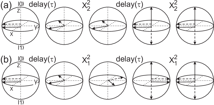
Mathematically, we can see how refocusing of couplings works using the fact that for all
| (42) |
which leads to
| (43) |
Replacing all with , the sequence works just the same. However, if we use sometimes and sometimes , we get the identity matrix only up to some phase shifts. Also, if we applied pulses on both qubits simultaneously, e.g. , the coupling would not be removed.
Fig. 12 gives insight in refocusing techniques in a multi-qubit system. Specifically, this scheme preserves the effect of , while effectively inactivating all the other couplings. The underlying idea is that a coupling between spins and acts “forward” during intervals where both spins have the same sign in the diagram, and acts “in reverse” whenever the spins have opposite signs. Whenever a coupling acts forward and in reverse for the same duration, it has no net effect.

Systematic methods for designing refocusing schemes for multi-qubit systems have been developed specifically for the purpose of quantum computing. The most compact scheme is based on Hadamard matrices Leung00a; Jones99a. A Hadamard matrix of order , denoted by , is an matrix with entries , such that
| (44) |
The rows are thus pairwise orthogonal, and any two rows agree in exactly half of the entries. Identifying and with and as in the diagram of Fig. 12, we see that gives a valid decoupling scheme for spins using only time intervals. An example of is
| (45) |
If we want the coupling between one pair of qubits to remain active while removing the effect of all other couplings, we can simply use the same row of for those two qubits.
does not exist for all , but we can always find a decoupling sequence for qubits by taking the first rows of , with the smallest integer that satisfies with known . From the properties of Hadamard matrices, we can show that is always close to 1 Leung00a. So decoupling schemes for spins require time intervals and no more than pulses.
Another systematic approach to refocusing sequences is illustrated via the following 4-qubit scheme Linden99c:
| (46) |
For every additional qubit, the number of time intervals is doubled, and pulses are applied to this qubit after the first, third, fifth, time interval. The advantage of this scheme over schemes based on Hadamard matrices, is that it does not require simultaneous rotations of multiple qubits. The main drawback is that the number of time intervals increases exponentially.
We end this subsection with three additional remarks. First, each qubit will generally be coupled to no more than a fixed number of other qubits, since coupling strengths tend to decrease with distance. In this case, all refocusing schemes can be greatly simplified Linden99c; Leung00a; Jones99a.
Second, if the forward and reverse evolutions under are not equal in duration, a net coupled evolution takes place corresponding to the excess forward or reverse evolution. In principle, therefore, we can organize any refocusing scheme such that it incorporates any desired amount of coupled evolution for each pair of qubits.
Third, refocusing sequences can also be used to remove the effect of terms in the Hamiltonian. Of course, these terms vanish in principle if we work in the multiply rotating frame (see Eq. 27). However, there may be some spread in the Larmor frequencies, for instance due to magnetic field inhomogeneities. This effect can then be reversed using refocusing pulses, as is routinely accomplished in spin-echo experiments (section V.1.4).
III.1.5 Pulse sequence simplification
There are many possible pulse sequences which in an ideal world result in exactly the same unitary transformation. Good pulse sequence design therefore attempts to find the shortest and most effective pulse sequence that implements the desired transformations. In section IV, we will see that the use of more complex pulses or pulse sequences may sometimes increase the degree of quantum control. Here, we look at three levels of pulse sequence simplification.
At the most abstract level of pulse sequence simplification, careful study of a quantum algorithm can give insight in how to reduce the resources needed. For example, a key step in both the modified Deutsch-Jozsa algorithm Cleve98a and the Grover algorithm Grover97a can be described as the transformation , where is set to , so that the transformation in effect is . We might thus as well leave out the last qubit as it is never changed.
At the next level, that of quantum circuits, we can use simplification rules such as those illustrated in Fig. 13. In this process, we can fully take advantage of commutation rules to move building blocks around, as illustrated in Fig. 14. Furthermore, gates which commute with each other can be executed simultaneously. Finally, we can take advantage of the fact that most building blocks have many equivalent implementations, as shown for instance in Fig. 15.

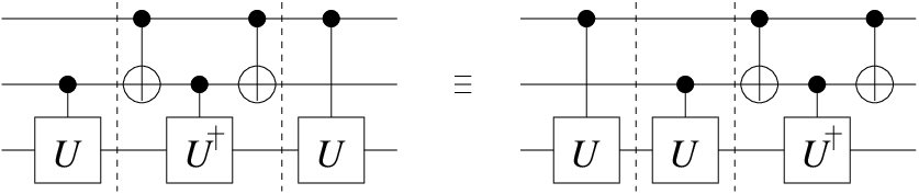

Sometimes, a quantum gate may be replaced by another quantum gate, which is easier to implement. For instance, refocusing sequences (section III.1.4) can be kept simple by examining which couplings really need to be refocused. Early on in a pulse sequence, several qubits may still be along , in which case their mutual couplings have no effect and thus need not be refocused. Similarly, if a subset of the qubits can be traced out at some point in the sequence, the mutual interaction between these qubits does not matter anymore, so only their coupling with the remaining qubits must be refocused. Fig. 16 gives an example of such a simplified refocusing scheme for five coupled spins.

More generally, the relative phases between the entries in the unitary matrix describing a quantum gate are irrelevant when the gate acts on a diagonal density matrix. In this case, we can for instance implement a cnot simply as rather than the sequence of Eq. 41.
At the lowest level, that of pulses and delay times, further simplification is possible by taking out adjacent pulses which cancel out, such as and (an instance of the first simplification rule of Fig. 13), and by converting “difficult” operations to “easy” operations.
Cancellation of adjacent pulses can be maximized by properly choosing the pulse sequences for subsequent quantum gates. For this purpose, it is convenient to have a library of equivalent implementations for the most commonly used quantum gates. For example, two equivalent decompositions of a cnot12 gate (with ) are
| (47) |
as in Eq. 41, and
| (48) |
Similarly, two equivalent implementations of the hadamard gate on qubit 2 are
| (49) |
and
| (50) |
Thus, if we need to perform a hadamard operation on qubit 2 followed by a cnot12 gate, it is best to choose the decompositions of Eqs. 47 and 50, such that the resulting pulse sequence,
| (51) |
simplifies to
| (52) |
An example of a set of operations which is easy to perform is the rotations about . While the implementation of rotations in the form of three RF pulses (Eq. 38) takes more work than a rotation about or , rotations about need in fact not be executed at all, provided the coupling Hamiltonian is of the form , as in Eq. 27. In this case, rotations commute with free evolution under the system Hamiltonian, so we can interchange the order of rotations and time intervals of free evolution. Using equalities such as
| (53) |
we can also move rotations across and rotations, and gather all rotations at the end or the beginning of a pulse sequence. At the end, rotations do not affect the outcome of measurements in the usual , “computational” basis. Similarly, rotations at the start of a pulse sequence have no effect on the usually diagonal initial state. In either case, rotations do then not require any physical pulses and are in a sense “for free” and perfectly executed. Indeed, rotations simply define the reference frame for and and can be implemented by changing the phase of the reference frame throughout the pulse sequence.
It is thus advantageous to convert as many and rotations as possible into rotations, using identities similar to Eq. 38, for example
| (54) |
A key point in pulse sequence simplification of any kind is that the simplification process must itself be efficient. For example, suppose an algorithm acts on five qubits with initial state and outputs the final state . The overall result of the algorithm is thus that qubit is flipped and that qubit is placed in an equal superposition of and . This net transformation can obviously be obtained immediately by the sequence . However, the effort needed to compute the overall input-output transformation generally increases exponentially with the problem size, so such extreme simplifications are not practical.
III.1.6 Time-optimal pulse sequences
Next to the widely used but rather naive set of pulse sequence simplification rules of the previous subsection, there exist powerful mathematical techniques for determing the minimum time needed to implement a quantum gate, using a given system and control Hamiltonian, as well as for finding time-optimal pulse sequences Khaneja01a. These methods build on earlier optimization procedures for mapping an initial operator onto a final operator via unitary transformations Sorenson89a; Glaser98a, as in coherence or polarization transfer experiments, common tasks in NMR spectroscopy.
The pulse sequence optimization technique expresses pulse sequence design as a geometric problem in the space of all possible unitary transformations. The goal is to find the shortest path between the identity transformation, , and the point in the space corresponding to the desired quantum gate, , while travelling only in directions allowed by the given system and control Hamiltonian. Let us call the set of all unitaries that can be produced using the control Hamiltonian only. Next we assume that the terms in the control Hamiltonian are much stronger than the system Hamiltonian (as we shall see in section III.2.2, this assumption is valid in NMR only when using so-called hard, high-power pulses). Then, starting from , any point in can be reached in a negligibly short time, and similarly, can be reached in no time from any point in the coset , defined by . Evolution under the system Hamiltonian for a finite amount of time is required to reach the coset starting from . Finding a time-optimal sequence for thus comes down to finding the shortest path from to , allowed by the system Hamiltonian.
Such optimization problems have been extensively studied in mathematics Brockett81a, and have been solved explicitly for elementary quantum gates on two coupled spins Khaneja01a and a three-spin chain with nearest-neighbour couplings Khaneja02a. For example, a sequence was found for producing the trilinear propagator from the system Hamiltonian in a time , the shortest possible time Khaneja02a. This propagator is the starting point for useful quantum gates such as the doubly-controlled not or toffoli gate. The standard quantum circuit approach, in comparison, would yield a sequence of duration (it uses only one coupling at a time while refocusing the other coupling), and the common NMR pulse sequence has duration .
Clearly, the time needed to find a time-optimal pulse sequence increases exponentially with the number of qubits, , involved in the transformation, since the unitary matrices involved are of size . Therefore, the main use of the techniques presented here lies in finding efficient pulse sequences for building blocks acting on only a few qubits at a time, which can then be incorporated in more complex sequences acting on many qubits by adding appropriate refocusing pulses to remove the couplings with the remaining qubits. While the examples given here are for the typical NMR system and control Hamiltonian, the approach is completely general and may be useful for other qubit systems too.
III.2 Experimental Limitations
Many years of experience have taught NMR spectroscopists that while the ideal control techniques described above are theoretically attractive, they neglect important experimental artifacts and undesired Hamiltonian terms which must be addressed in any actual implementation. First, a pulse intended to selectively rotate one spin will to some extent also affect the other spins. Second, the coupling terms cannot be switched off in NMR. During time intervals of free evolution under the system Hamiltonian, the effect of these coupling terms can easily be removed using refocusing techniques (section III.1.4), so long as the single-qubit rotations are perfect and instantaneous. However, during RF pulses of finite duration, the coupling terms also distort the single-qubit rotations. In addition to these two limitations arising from the NMR system and control Hamiltonian, a number of instrumental imperfections cause additional deviations from the intended transformations.
III.2.1 Cross-talk
Throughout the discussion of single- and two-qubit gates, we have assumed that we can selectively address each qubit. Experimentally, qubit selectivity could be accomplished if the qubits are well-separated in space or, as in NMR, in frequency. In practice, there will usually be some cross-talk, which causes an RF pulse applied on resonance with one qubit to slightly rotate another qubit, or shift its phase. Cross-talk effects are even more complex when two or more pulse are applied simultaneously.
The frequency bandwidth over which qubits are rotated by a pulse of length is roughly speaking of order . Yet, since the qubit response to an RF field is not linear (it is sinusoidal in ), the exact frequency response cannot be computed using Fourier theory.
For a constant amplitude (rectangular) pulse, the unitary transformation as a function of the detuning is easy to derive analytically from Eqs. 22 and 23. Alternatively, we can exponentiate the Hamiltonian of Eq. 21 to get directly. An example of a qubit response to a rectangular pulse is shown in Fig. 17.

It is evident from Fig. 17 that short rectangular pulses (known as “hard” pulses) excite spins over a very wide frequency range. The frequency selectivity of a pulse can of course be increased by increasing while lowering accordingly (thus creating what is known as a “soft” pulse), but decoherence effects become more severe as the pulses get longer. Fortunately, as we will see in sections IV.1 and IV.2, the use of shaped and composite pulses can dramatically improve the frequency selectivity of the RF excitation.
Even if a pulse is designed not to produce any net or rotations of spins outside a specified frequency window, the presence of RF irradiation during the pulse still causes a shift in the precession frequency of spins at frequencies well outside the excitation frequency window Emsley90a. As a result, each spin accumulates a spurious phase shift during RF pulses applied to spins at nearby frequencies.
This effect is related to the Bloch-Siegert shift mentioned in section II.2.1, and is known as the transient generalized Bloch-Siegert shift in the NMR community. It is related to the AC Stark effect in atomic physics. At a deeper level, the acquired phase can be understood as an instance of Berry’s phase Berry84a: the spin describes a closed trajectory on the surface of the Bloch sphere and thus returns to its initial position, but it acquires a phase shift proportional to the area enclosed by its trajectory.
The frequency shift is given by
| (55) |
(provided ), where is the original Larmor frequency (in the absence of the RF field). In typical NMR experiments, the frequency shifts can easily reach several hundred Hz in magnitude. We see from Eq. 55 that the Larmor frequency shifts up if and shifts down if .
Fortunately, the resulting phase shifts can be easily computed in advance for each possible spin-pulse combination, if all the frequency separations, pulse amplitude profiles and pulse lengths are known. The unintended phase shifts can then be compensated for during the execution of a pulse sequence by inserting appropriate , which can be executed at no cost, as we saw in section III.1.5.
Cross-talk effects are aggravated during simultaneous pulses, applied to two or more spins with nearby frequencies and (say ). The pulse at then temporarily shifts the frequency of spin to . As a result, the pulse on spin , if applied at , will be off-resonance by an amount . Analogously, the pulse at is now off the resonance of spin 1 by . The resulting rotations of the spins deviate significantly from the intended rotations.
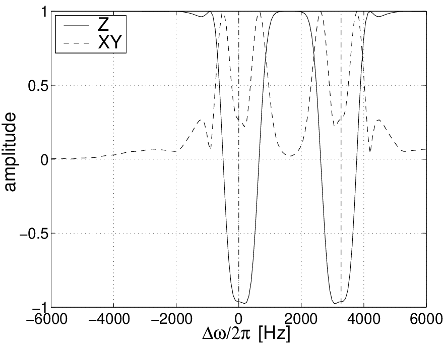
The detrimental effect of the Bloch Siegert shifts during simultaneous pulses is illustrated in Fig. 18, which shows the simulated inversion profile for a spin subject to two simultaneous 180∘ pulses separated by 3273 Hz. The centers of the inverted regions have shifted away from the intended frequencies and the inversion is incomplete, which can be seen most clearly from the substantial residual -magnetization () over the whole region intended to be inverted. Note also that since the frequencies of the applied pulses are off the spin resonance frequencies, complete inversion cannot be achieved no matter what tip angle is chosen (see section II.2.2).
In practice, simultaneous soft pulses at nearby frequencies have been avoided in NMR Linden99a or the poor quality of the spin rotations was accepted. Pushed by the stringent requirements of quantum computation, several techniques have meanwhile been invented to generate accurate simultaneous rotations of spins at nearby frequencies (sections IV.1.2 and IV.2.2).
III.2.2 Coupled evolution
The spin-spin couplings in a molecule are essential for the implementation of two-qubit gates (section III.1.3), but they cannot be turned off and are thus also active during the RF pulses, which are intended to be just single-qubit transformations. Unless is much stronger than the coupling strength, the interactions strongly affect the intended nutation. For couplings of the form , the effect is similar to the off-resonance effects illustrated in Fig. 7: the coupling to another spin shifts the spin frequency to , so a pulse sent at hits the spin off-resonance by .
In practice, -coupling terms can only be neglected for short, high-power pulses used in heteronuclear spin systems: typically Hz while is up to kHz. For low-power pulses, often used in homonuclear spin systems, can be of the same order as and coupling effects become prominent. The coupling terms also lead to additional complications when two qubits are pulsed simultaneously. In general, the qubits become partially entangled Kupce95a.
As was the case for cross-talk, NMR spectroscopists have developed special shaped and composite pulses to compensate for coupling effects during RF pulses while performing spin-selective rotations. In recent years, the use of such pulses has been extended and perfected for quantum computing experiments (sections IV.1 and IV.2).
III.2.3 Instrumental errors
A number of experimental imperfections lead to errors in the quantum gates. In NMR, the most common imperfections are inhomogeneities in the static and RF magnetic field, pulse length calibration errors, frequency offsets, and pulse timing and phase imperfections.
The static field in modern NMR magnets can be made homogeneous over the sample volume (a cylinder mm in diameter and cm long) to better than part in . This amazing homogeneity is obtained by meticulously adjusting the current through a set of so-called “shim” coils, which compensate for the inhomogeneities produced by the large solenoid. At MHz, linewidths of Hz can thus be obtained, corresponding to a dephasing time constant (see Section V.1.2) of s. In the course of long pulse sequences (of order s), even the tiny remaining inhomogeneity would therefore have a large effect, so its effect must be reversed using refocusing sequences (section III.1.4)
The RF field homogeneity is typically very poor, due to constraints on the geometry of the RF coils: the envelope of Rabi oscillations (section V.1.1) often decays by as much as per rotation, corresponding to a quality factor of only . In sequences containing only a few pulses, this is not problematic, but in multiple-pulse experiments, the RF field inhomogeneity is often the dominant source of errors and signal loss.
Imperfect pulse length calibration has an effect similar to inhomogeneity: the qubit rotation angle is different than was intended. Only the correlation time for the error is different. Miscalibrations are constant throughout an experiment, whereas the RF field experienced by any given molecule changes on the timescale of diffusion through the sample volume.
Frequency offsets occur in different contexts. In traditional NMR experiments, the Larmor frequencies are often not known in advance. RF pulses are then expected to rotate the spins over a wide range of frequencies, quite the opposite case of quantum computing, where the Larmor frequencies are precisely known and rotations should be spin-selective. However, we have seen earlier that coupling terms act as a frequency offset of one spin, which depends on the state of the other spin. Qubit-selective rotations of qubit thus require a uniform rotation over a range .
Various approaches have been developed to reduce the sensitivity of RF pulses and pulse sequences to these instrumental errors, sometimes in combination with solutions to cross-talk and coupling artifacts. These advanced techniques are the subject of the next section.
IV Advanced pulse techniques
The accuracy of quantum gates that can be achieved using the simple pulse techniques of the previous section is unsatisfactory when applied to multi-spin systems, where the given NMR system and control Hamiltonian lead to undesired cross-talk and coupling effects. In addition, the available instrumentation can only imperfectly approximate ideal pulse amplitudes, timings, and phases, for realistic sample geometries and coil configurations, and any real molecule includes additional Hamiltonian terms such as couplings to the environment, which are undesired. Nevertheless, extremely precise control can be achieved despite these imperfections, and this is accomplished using the art of shaped pulses, composite pulses and average Hamiltonian theory, the subject of this second major section of this review.
These advanced techniques are based on the assumption that errors are, at least on some accessible timescale, systematic, rather than random. This assumption clearly holds for the terms in the ideal NMR Hamiltonian of Eqs. 27 and 28, and applies also to most instrumental errors. Then, by using the special properties of evolution in unitary groups, such as the which describes the space of operators acting on qubits, the systematic errors can in principle be canceled out.
IV.1 Shaped pulses
The amplitude and phase profile of RF pulses can be specially tailored in order to ease the cross-talk and coupling effects discussed in sections III.2.1 and III.2.2. In practice, the pulse is divided in a few tens to many hundreds of discrete time slices; to achieve an arbitrarily shaped pulse, it suffices to control the amplitude and phase of the slices separately. Furthermore, multiple shaped pulses applied at various frequencies can be combined into a single pulse shape, since a linear vector sum of pulse slices also results in a valid pulse. Here, we consider simple amplitude and phase shaped pulses.
IV.1.1 Amplitude profiles
The frequency selectivity of RF pulses can be much improved compared to standard rectangular pulses with sharp edges, by using pulse shapes which smoothly modulate the pulse amplitude with time. Such pulses are typically specially designed to excite or invert spins over a limited frequency region, while minimizing and rotations for spins outside this region Freeman98a; Freeman97a.
Furthermore, specialized pulse shapes exist which minimize the effect of couplings during the pulses. Such self-refocusing pulses Geen91a take a spin over a complicated trajectory in the Bloch sphere, in such a way that the net effect of couplings between the selected and non-selected spins is reduced (Fig. 19). It is as if those couplings are only in part or even not at all active during the pulse (couplings between pairs of non-selected spins will still be fully active but their effect can be removed using standard refocusing techniques III.1.4). As a general rule, it is relatively easy to make pulses self-refocusing, but much harder to do so for pulses.

The self-refocusing behavior of certain shaped pulses can be intuitively understood to some degree. Nevertheless, many actual pulse shapes have been the result of numerical optimizations. Often, the pulse shape is expressed in a basis of several functions, for instance a Fourier series Geen91a,
| (56) |
and the weights of the basis functions, and , are optimized using numerical routines such as simulated annealing.
Comparison of the performance of various pulse shapes is facilitated by computing the corresponding spin responses. This is most easily done by concatenating the unitary operators of each time slice of the shaped pulse, as the Hamiltonian is time-independent within each time slice. Fig. 20 presents the amplitude profile and pulse response for three standard pulse shapes of equal duration, illustrating that different pulse shapes produce strikingly different spin response profiles.

Properties relevant for choosing a pulse shape include:
- •
frequency selectivity: product of excitation bandwidth and pulse length (lower is more selective),
- •
transition range: the width of the transition region between the selected and non-selected frequency region,
- •
power: the peak power required for a given pulse length and tip angle (lower is less demanding),
- •
self-refocusing behavior: degree to which the coupling between the selected spin and other spins are refocused (the signature for self-refocusing behavior is a flat top in the excitation profile),
- •
robustness to experimental imperfections such as pulse length errors,
- •
universality: whether the pulse performs the intended rotation for arbitrary input states or only for specific input states.
Table 2 summarizes these properties for a selection of widely used pulse shapes. Only universal pulses (also known as general-rotation pulses) are included in the table, since quantum computations must work for any input state.
| selec- | transition | self- | robust- | ||
|---|---|---|---|---|---|
| tivity | range | power | refocusing | ness | |
| Rectangular | poor | very wide | minimal | no | good |
| Gauss 90 | excellent | wide | low | fair | good |
| Gauss 180 | excellent | wide | low | fair | good |
| Hrm 90 | moderate | moderate | average | good | fair |
| Hrm 180 | good | moderate | average | very good | fair |
| uburp 90 | poor | narrow | high | excellent | poor |
| reburp180 | poor | narrow | high | excellent | poor |
| av 90 | fair | moderate | average | good | fair |
Obviously, no single pulse shape optimizes for all properties simultaneously, so pulse shape design consists of finding the optimal trade-off for the desired application. For quantum computing experiments, we can select molecules with large chemical shifts, so sharp transition regions are not so important. Furthermore, the probe and spectrometer can deal with relatively high powers. The crucial parameters are the self-refocusing behavior, the selectivity (short, selective pulses minimize decoherence) and to some extent the robustness.
It is also possible to start from a desired frequency response, and invert the transformation to find the pulse shape that produces this response. Again, given the non-linear nature of the response, the inverse transformation is not given by a Fourier transform, but it can nevertheless be computed directly Pauly91a.
Even self-refocusing shaped pulses do generally not remove the coupling terms completely. Furthermore, when two spins are pulsed simultaneously with self-refocusing pulses, the refocusing effects are often destroyed Kupce95a. In both cases, the remaining coupled evolution that takes place during the pulses must be reversed at an earlier and/or later stage in the pulse sequence.
If we could decompose the evolution during an actual pulse into an idealized, instantaneous or rotation with no coupling present, followed and/or preceded by a time interval of free evolution, we could compensate for the coupling effects simply by adjusting the appropriate time intervals of free evolution in between the pulses (section III.1.4). However, and do not commute, so such a decomposition is not possible.
Nevertheless, the coupled evolution can still be unwound to first order Vandersypen01a; Knill00a, when a time interval of reverse evolution both before and after the pulse is used:
| (57) |
where is chosen such that the approximations are as good as possible according to some distance or fidelity measure (see section V.3). The optimal is usually close but not equal to . In comparison, a negative time interval only before or after the pulse,
| (58) |
is much less effective.
IV.1.2 Phase profiles
An alternative to amplitude shaping that is often useful is frequency or phase shaping. One specific phase shaping method utilizes fixed, small increments to the phase of successive slices of a pulse to achieve an excitation profile which is centered at a frequency which differs from the RF carrier frequency by , where is the duration of each time slice. This technique for shifting the RF frequency is known as phase-ramping Patt91a. We can express the effect of phase ramping mathematically by replacing Eq. 17 by
| (59) | |||||
The use of phase shifts thus permits us to obtain an RF field at a
different frequency than is generated by the signal generator.
Furthermore, the displaced frequency can be chosen different for every
pulse, and can even be varied in the course of a pulse.
A useful application of phase ramping lies in compensation for Bloch-Siegert effects during simultaneous pulses, where the RF applied at shifts the resonance frequency of spin to (Section III.2.1). The rotations of both spins can be significantly improved simply by shifting the RF excitation frequencies via phase ramping such that they track the shifts of the corresponding spin frequencies Steffen00a. In this way, the pulses are always applied on-resonance with the respective spins. The calculation of the frequency shift throughout a shaped pulse is straightforward and needs to be done only once, at the start of a series of experiments.
Fig. 21 shows the simulated inversion profiles for the same conditions as in Fig. 18, but this time using the frequency shift corrected scheme. The inversion profiles are clearly much improved and there is very little left-over magnetization. Simulations of the inversion profiles for a variety of pulse shapes, pulse widths and frequency separations, confirm that the same technique can be used to correct the frequency offsets caused by three or more simultaneous soft pulses at nearby frequencies. The improvement is particularly pronounced when the frequency window of the shaped pulse is two to eight times the frequency separation between the pulses Steffen00a.

IV.2 Composite pulses
Another practical method for compensating systematic control errors in NMR experiments is the application of a sequence of pulses instead of a single pulse. This method of composite pulses arises from the observation that concatenation of several pulses can produce more accurate rotations than is possible using just a single pulse, due to strategic cancellation of systematic errors and other unwanted systematic effects. Composite pulses work particularly well for compensating errors arising from the RF field inhomogeneity, frequency offsets, imperfect pulse length calibration, and other instrumental artifacts introduced in Section III.2.3. They leverage the ability to control one parameter precisely to compensate for the inability to control another parameter well. We describe two approaches to construction of composite pulses: an analytical method, and one employing numerical optimization.
IV.2.1 Analytical approach
The three parameters which characterize a hard pulse are its frequency offset , phase , and area , given by the product of the pulse amplitude and pulse duration (Section II.2.1). In terms of qubit operations, errors in these parameters translate directly into errors in the axis and angle of rotation, such that the actual operation applied is not the ideal of Eq.(29), but rather,
| (60) |
where is a function which characterizes the systematic error. For example, under and over-rotation errors caused by pulse amplitude miscalibration or RF field inhomogeneity may be described by , while RF phase errors may be described by , where is a fixed, but unknown parameter. The essence of the composite pulses technique is that a number of erroneous operations are concatenated, varying and , to obtain a final operation which is as independent of as possible. This is done without knowing .
This technique can be illustrated by considering the specific case of linear amplitude errors, in which
| (61) |
Let the goal be to obtain . Using as a measure of error the average gate fidelity, defined in Eq.(123), we find that , so the error is quadratic in for small . Consider, in contrast, the sequence
| (62) |
where denotes a rotation about the axis , and the choice is made. This sequence gives average gate fidelity , which is much better than for the single pulse, even for relatively large values of , as shown in Figure 22. The operation of the sequence is illustrated graphically in Fig. 23.

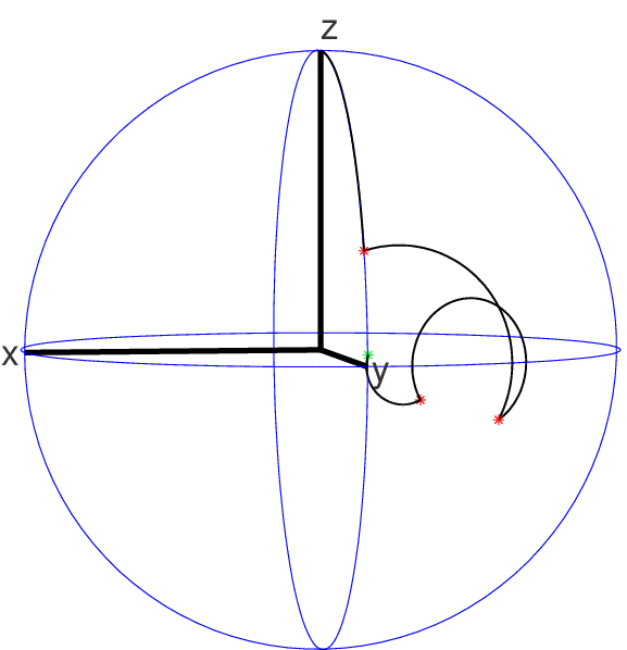
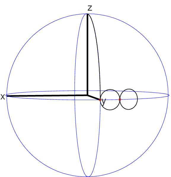
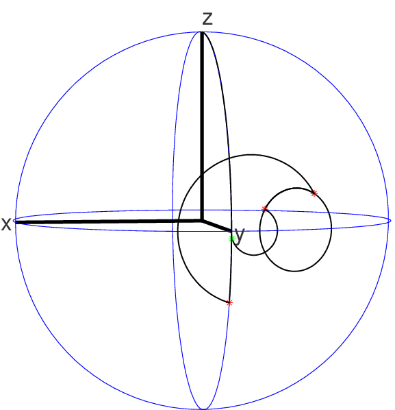
A few comments about this result are in order. This result is the best which has been presented in the literature to-date Cummins00a; Jones03b; Wimperis94a; currently, no pulse sequence which cancels out errors to higher order (for all possible initial states) has yet been published. It is also fairly general; approximates . Also, while composite pulses have been widely studied and employed in the art of NMR, this sequence is special in that it is universal (also termed fully-compensating or class ): the amount of error cancellation is independent of the starting state of the spin Tycko83a; Tycko85a. Other examples of such universal composite pulses are the sequence
| (63) |
which performs a rotation with compensation for pulse length errors, and
| (64) |
which performs a rotation compensating for off-resonance errors and to some extent for pulse length errors as well.
Earlier, in the original work which introduced the concept of composite pulses into NMR Levitt79a; Levitt86a, only limited pulse sequences were known, which only work for particular initial states; for example, there is the common , used to approximate . Figure 24 illustrates how this simple sequence removes the effect of errors in either the rotation angle or the rotation axis.


Systematic errors in the coupling strengths can also be tackled using composite rotations, in order to obtain accurate two-qubit gates. This was shown explicitly for the case of Ising couplings Jones03a.
Similar compensation of slowly-fluctuating errors can be achieved during a train of pulses, separated by time intervals of free evolution. The simplest instance of such a pulse train uses only pulses. Off-resonance effects in such pulses can be largely reversed by properly choosing the phases of the pulses. For instance, and at first sight surprisingly, the errors from off-resonant pulses roughly add up, while they largely compensate each other in . This cancellation can be appreciated via a simple Bloch sphere picture (Fig. 25). The remaining errors are further reduced for a properly chosen train of four pulses, , which performs markedly better than Levitt82a. Further reduction of the effect of off-resonance errors can be obtained by using even longer trains of pulses Levitt82a.


Evidently, quantum computing sequences are not as transparent as just a train of pulses. Surprisingly, even throughout a quantum computing sequence, the effect of RF inhomogeneities can be removed to a large extent Vandersypen00a, as illustrated in Fig. 26. After completion of a routine involving the equivalent of about 1350 pulses, the measured amplitude was about of the full amplitude. Without removal of the effect of RF inhomogeneity, the signal would have been buried in the noise very rapidly.

This level of error cancellation was achieved partly due to a judicious choice of the phases of the refocusing pulses. Nevertheless, a more detailed description and understanding of the error operators is needed in order to fully exploit the potential for error cancellation in arbitrary pulse sequences.
IV.2.2 Numerical optimization
The composite pulses we discussed in the previous subsection are designed to compensate for certain types of errors (mostly over- or underrotations and frequency offsets), and work even when the exact Larmor frequencies, spin-spin coupling strengths and the magnitude of the errors are unknown. This is the usual case in NMR spectroscopy. However, in quantum computing experiments, detailed knowledge of the system Hamiltonian is usually available and can be used to tailor the composite pulses to the system specifics, taking the degree of quantum control one step further.
Following the notation of Ref. Fortunato02a, we consider the concatenation of a number of rectangular pulses, each described by four parameters: the pulse duration , a constant amplitude , the transmitter frequency and the initial phase , where indexes the pulse. These parameters may be strongly modulated from one pulse to the next33 3 Jumps in the transmitter frequency can be conveniently realized with phase-ramping techniques; as discussed in Section IV.1.2, this is done by phase shifting the raw RF excitation in fixed increments per time so a different RF frequency is obtained. Via a numerical optimization procedure, the values of , , and are chosen such that the resulting net unitary evolution is as close as possible to the ideal unitary transformation , according to some fidelity measure (section V.3).
In practice, the number of time slices in the composite pulse is increased starting from one, until a satisfactory solution is found. While the fidelity function may have many local maxima and finding the global maximum may therefore take a long time, suitable algorithms such as the Nelder-Mead Simplex algorithm Nelder65a often succeed in finding a reasonably good solution. Furthermore, the optimization routine can incorporate penalties on high powers, large frequencies and negative or very long time periods, in order to prevent the algorithm from returning infeasible solutions.
Computation of uses the fact that the Hamiltonian during a fixed-amplitude RF pulse can be made time independent by transforming into a reference frame rotating at the transmitter frequency, as we have seen in section II.2.2. We will call the effective Hamiltonian in the frame rotating at during segment . Given that may be different for every segment of the pulse, it is most convenient to transform back to a common reference frame at the end of every time slice. This can be the frame of the raw RF frequency, or the laboratory frame of the -spin system. In the lab frame, the time evolution during segment is described by
| (65) |
Since all are expressed in the same reference frame, we can simply multiply them together to get , and compare the result directly with , expressed in the laboratory frame as well.
Two representative examples of composite pulses designed for spin-selective rotations in homonuclear spin systems are given in Fig. 27. The gate fidelity (section V.3.2) obtained with these two pulses is displayed in Fig. 28. Naturally, the fidelity is close to unity only near the resonance frequencies for which the gate was designed to work.


Composite pulses can thus effectively generate accurate single- and multiple-qubit Hamiltonians, using detailed knowledge of the system Hamiltonian, and only limited knowledge about the errors. Often, however, full knowledge of the system parameters is not available, and thus methods beyond composite pulses must be employed.
IV.3 Average-Hamiltonian theory
The average-Hamiltonian formalism offers a versatile framework for understanding how to effectively create or remove arbitrary terms in the Hamiltonian by periodic perturbations, without requiring full knowledge of the system dynamics. The refocusing sequences presented in section III.1.4 and more general multiple-pulse sequences designed to neutralize the effect of dipole-dipole couplings can be explained within this framework. Reduction of full dipole-dipole coupling given by Eq. 11 to the simplified forms of Eqs. 12 and 13 can also be understood with average-Hamiltonian theory.
Following Ref. Ernst87a, we first introduce the Magnus expansion and then see how we can modify a time-independent Hamiltonian via a time-dependent perturbation. We use two concrete examples to illustrate the concepts.
IV.3.1 The Magnus expansion
The essence of average-Hamiltonian techniques is that the evolution under a time-dependent Hamiltonian can be described by an effective evolution under a time-independent average Hamiltonian , under two conditions Haeberlen68a; Ernst87a: (1) is periodic and (2) the observation is stroboscopic and synchronized with the period of .
We can then calculate exactly from
| (66) |
by diagonalizing and taking the logarithm of the resulting eigenvalues Nielsen00b.
In practice, it is often more convenient to compute approximately. Let us assume that is piecewise constant (the analysis can be easily generalized to the case of continuously changing Hamiltonians Ernst87a): for , and , so
| (67) |
Repeated application of the Baker-Campbell-Hausdorff relation
| (68) | |||||
gives
| (69) |
where
| (70) | |||||
| (71) | |||||
and so forth. This expansion, called the Magnus expansion Magnus54a, forms the basis of average-Hamiltonian theory.
IV.3.2 Multiple-pulse decoupling
Let us consider a pulse sequence of infinitesimally short pulses separated by time intervals of free evolution under the system Hamiltonian , and such that (for pulses of finite length, the duration of the pulses must also be included in the average). The pulses correspond to basis transformations, and we can thus describe the system evolution via a sequence of time intervals of free evolution under the Hamiltonian , with
| (72) | |||||
| (73) | |||||
| (74) |
and so forth. Note that the order in which the are applied to is reversed and that the themselves are reversed as well. If we let , then the overall transformation is given by
| (75) |
We can now use the Magnus expansion of Eq. 69 and Eqs. 70-71, where we replace by , to obtain the average Hamiltonian which describes the net time evolution during . The zeroth order average Hamiltonian is given by
| (76) |
The crux of average Hamiltonian theory is that by properly choosing the pulse , we can ensure that contain only the desired terms.
Sophisticated pulse sequences Mehring83a can also remove undesired contributions from the higher-order terms in the expansion, although this is generally harder since contain cross-terms between the various . The commutators involved in the higher-order terms do become smaller for shorter cycle times, though, so fast cycles result in better averaging.
We also point out that pulse sequences which satisfy
| (77) |
or equivalently
| (78) |
contain no contributions of odd orders to ,
| (79) |
and thus perform significantly better than other sequences.
Let us now illustrate the operation of multiple-pulse decoupling via two examples. First, the original multiple-pulse sequence for removal of dipole-dipole interactions is the wahuha-4 sequence Waugh68a,
| (80) |
where the pulses are applied to all qubits involved, stands for free evolution under the system Hamiltonian for a duration , and the unitaries are ordered from right to left, as usual. The pulses rotate the Zeeman terms in the Hamiltonian from to , , , and back to (see Eqs. 72-74) for a duration , , , and , respectively. The zeroth order average Zeeman term is thus oriented along , with strength scaled down by a factor . The dipolar Hamiltonian of Eq. 12 goes through the forms , and for equal durations, and is thus zero on average.
By selectively not pulsing specific qubits, it is also possible to reintroduce some of the couplings as desired. In Fig. 12, we already saw explicitly how to do this for couplings.
A second example is an extension of the conventional spin-echo sequence (Section V.1.4) to three component spin-echoesAugustine97a. In conventional echo sequences, pulses about or remove the effect of a Hamiltonian of the form . Now we ask ourselves what sequence of pulses would freeze the evolution under a Hamiltonian of the form
| (81) |
where are arbitrary coefficients. We can use Eq. 76 to verify that the sequence
| (82) |
or equivalently, after simplification,
| (83) |
gives a zeroth order average Hamiltonian , and thus in effect corresponds to a three-component echo sequence. Another way to show this is to note that
| (84) | |||||
| (85) | |||||
| (86) |
Clearly, , and so the sequence of Eq. 82 gives, to zeroth order, no net evolution. Again, if is sufficiently short, the higher order contributions will be negligible.
IV.3.3 Reversing errors due to decoherence
Can we apply multiple-pulse sequences to reverse the effect of interactions of a qubit with degrees of freedom in the environment? It is not clear a priori that this is possible: standard average-Hamiltonian theory assumes that we can manipulate both interacting particles involved, for instance via RF pulses. However, we have no control of degrees of freedom in the environment.
Remarkably, it is actually possible to remove the effect of unwanted interactions with degrees of freedom in the environment, even when applying operations to the system only Viola98a; Viola99a; Vitali99a; Duan99a, provided the control operations are applied faster than the fluctuations. Knowledge about the nature of the interactions can be applied to simplify the sequence of decoupling operations, and such knowledge can even be experimentally extracted Byrd03a, in part using a procedure known as process tomography, described in Section V.2.2.
If the fluctuations are faster than the accessible control operations, errors can be corrected using quantum error correction Shor95a; Steane96a; Nielsen00b, or they can prevented by encoding the qubits in a subspace which is not affected by decoherence Lidar98a; Zanardi98a. This is discussed further in Section V.4.
V Evaluation of quantum control
The pulse control methods presented in the last two sections can have impressive performance, but this is very much contingent on having an accurate model of the system under control. A variety of techniques have been used in NMR to characterize the system dynamics and to evaluate the performance of control sequences. In this last section, we review some of these techniques, beginning with a set of standard experiments to determine how quantum a qubit system is, then proceeding to tomographic methods for fully characterizing system dynamics, and concluding with fidelity metrics for control, and implications these have for scalability to control over large systems.
V.1 Standard experiments
In NMR spectroscopy as in atomic physics, a number of standard experiments serve to test the quantum-mechanical behavior of a given system, and to determine the extent of its isolation from the environment (see Section II.3), in terms of its phase coherence time and its energy relaxation time , as well as the decay time in the rotating frame .
V.1.1 Coherent oscillations driven by a resonant field
The dynamics of a single spin, driven resonantly by a coherent field, were presented in sections II.2.1 and II.2.2. From Eq. 37, we have that in the ideal case the RF field induces transitions from to , where a qubit initially in will be found in after an RF pulse of duration with probability
| (87) |
The probability initially increases over time, until it reaches a maximum and then decreases again, by stimulated emission, a cycle which keeps repeating itself.
Such oscillations of a two-level quantum system driven by a resonant field are known as Rabi oscillations Rabi37a, and the Rabi frequency is proportional to the amplitude of the control field. Observation of Rabi oscillations is usually accepted as a signature of quantum coherent behavior.
In reality, the envelope of the Rabi oscillation signal is always damped, due to decoherence as well as instrumental imperfections; measurement of this decay time is useful, and known as a nutation experiment. In NMR, the Rabi decay time is often much shorter than the intrinsic phase randomization time constant , due to the inhomogeneity of the RF field driving the Rabi oscillation, across the macroscopic sample. In other systems, the Rabi decay time may be longer than , because (1) a long pulse can be seen as a concatenation of many pulses, which can have a refocusing effect (section III.1.4), and (2) the qubit is near , where phase randomization has no effect, for roughly half the time during Rabi oscillations.
Coherent oscillations driven by a resonant field have been observed in NMR and in many atomic systems for a long time. Recently, however, observations of such coherent dynamics have been made in other qubit systems, including systems made from Josephson junctions Nakamura99a, in molecular vibrational states Vala02a; Tesch02a, and excitons in semiconductor quantum dots Stievater01a.
V.1.2 Coherent oscillations initiated by a kick
A quantum system starting off in a state which is not an eigenstate of the (static) system Hamiltonian, will precess about the quantization axis of the system Hamiltonian, a motion known as Larmor precession (e.g. Section II.1.1). Such a situation could be realized by abruptly changing the system Hamiltonian, e.g. by suddingly applying a strong static field along instead of along . Alternatively, and more realistically in NMR, Larmor precession can be initiated by suddenly kicking the qubit out of the Hamiltonian eigenbasis. For a nuclear spin with Hamiltonian (as in Eq. 1), this is done by applying a RF pulse, causing a transition for instance from to , which initiates the time evolution
| (88) |
as illustrated in Fig. 2. Like Rabi oscillations, the observation of Larmor precession is also a signature of quantum coherent behavior.
The Larmor precession is also damped, but in contrast to the Rabi decay time, the Larmor decay time, termed , is never longer than . Usually, ; in particular, for NMR,
| (89) |
where is the dephasing time constant due to static magnetic field inhomogeneities or other instrumental imperfections.
Larmor oscillations initiated by a kick have been observed recently in a variety of systems, including those driven resonantly mentioned earlier, and in addition a system of charges in coupled quantum dots Hayashi03a. The oscillations can be observed directly if the measurement basis lies in the plane, as is the case in NMR. If the measurement takes place along , we must first change basis via a second pulse.
V.1.3 Ramsey Interferometry
The double-pulse experiment
| (90) |
where time goes from right to left (as always, for unitary transformations given in this article), and denotes a free evolution period, under the evolution operation . This is known as a Ramsey interference experiment Ramsey50a. Originally, this “method of separated oscillatory fields” was applied to electronic states of molecular beams traversing through two microwave excitation zones. In NMR, two pulses are involved, separated by a delay time . Ramsey interference is most naturally described in the rotating frame of the RF. If the qubit starts off along , the first pulse rotates it to . Then the qubit precesses about for a time . Finally the second pulse rotates the component of the qubit state to . Components along at the end of the interval remain along after the second pulse.
If only a single qubit is considered and the RF field is exactly on-resonance with the qubit precession, the qubit stays in place in the rotating frame during the time interval in between the two pulses, and the final state does not vary with . However, if the RF and the qubit are detuned in frequency by , both the and the components of the final state display a beating pattern as a function of , the so-called Ramsey fringes. The decay time of the envelope of the Ramsey fringes is , the same as that for Larmor precession.
V.1.4 Measurement of
The intrinsic time can be extracted in an experiment which is based on Larmor or Ramsey experiments. Certain imperfections which cause the Ramsey or Larmor decay time to be smaller than can be removed by applying refocusing sequences.
The simplest instance of such a refocusing sequence consists of a single pulse applied halfway during the time interval of free evolution initiated by an initial pulse. The entire sequence is thus
| (91) |
A second pulse should be added at the end if the measurement takes place in the basis. In multi-spin systems, the pulses must be applied selectively to one spin, in order to measure the of that spin.
The refocusing pulse removes not only simple scalar spin-spin couplings, as described in section III.1.4, but also undoes the effect of spatial variations of the static magnetic field along . Such field inhomogeneities make spins in different regions of the sample progressively get out of phase with each other during the first time interval . As a result, their magnetic moments cancel each other out and the NMR signal vanishes. Provided the magnetic field variations are constant throughout the experiment, all the spins get exactly in-phase again (now along ) by the end of the second time interval , because of the refocusing pulse. As a result, the signal recovers, producing the well-known spin-echo. A generalization of this technique known as three-component refocusing (Section IV.3.2), undoes effects from any static spin Hamiltonian terms.
The echo signal decays as a function of , and the decay time constant is a measure of . However, terms in the Hamiltonian fluctuating on a timescale shorter than are not removed by a single refocusing pulse. Their effect can still be removed if the fluctuations are slow compared to and a train of refocusing pulses is applied, each preceded and followed by a time interval of free evolution. This so-called Carr-Purcell sequence Carr54a,
| (92) |
produces a first echo along after , a second echo along after , a third along after , and so forth. The magnitude of the echo signal decays exponentially throughout this sequence and the echo signal left at the end of this sequence decreases exponentially as a function of the total time . To the extent that slow fluctuations in the Hamiltonian have been refocused, the decay time constant is the intrinsic .
As we have seen in Section III of this review, small but fixed errors in the pulse amplitude or duration may accumulate throughout a multiple-pulse sequence such as the Carr-Purcell sequence. However, if the phase of the refocusing pulses is shifted by with respect to the initial pulse, pulse length errors are compensated on even-numbered echoes and are thus not cumulative. In this sequence,
| (93) |
known as the Carr-Purcell-Meiboom-Gill or CPMG sequence Meiboom58a, the echoes appear all along . Again, the decay time constant of the echo signal gives .
Since indicates for how long a qubit can remain phase coherent, it is usually called the coherence time, although the terms phase randomization time, dephasing time and transverse relaxation time, are also used. In NMR, is also known as the spin-spin relaxation time. In any case, is an important number for evaluating the potential of quantum computers, as the ratio of over the typical duration of a quantum logic gate expresses the number of operations that can be completed coherently.
V.1.5 Measurement of
Energy exchange with the environment makes a qubit which is out of equilibrium gradually return to thermal equilibrium. In thermal equilibrium, the qubit is in a statistical mixture of and , with probabilities set by the temperature and the energy difference between and . The time constant of this equilibration process, , is often called the energy relaxation time, the longitudinal relaxation time or simply the relaxation time. In NMR, is often termed the spin-lattice relaxation time.
Two standard experiments for measuring are inversion recovery and saturation recovery. The sequence for the inversion recovery experiment is
| (94) |
The pulse inverts the and probabilities, then during time , relaxation takes place, and finally a read-out pulse is applied if necessary (i.e. when the measurement basis is in the plane). In saturation recovery, a strong RF field is applied for a long enough time such that it saturates the qubit transition and equalizes the and probabilities. As in inversion recovery, the original and populations are altered, and we can monitor the populations return to their equilibrium value as a function of . The time constant of this equilibration process is .
Note that both the inversion recovery and saturation recovery experiments bring the qubit out of equilibrium, but to a state which has no coherence. As a result, phase randomization does not affect the equilibration process — we measure purely the effect of energy exchange with the bath. In contrast, Ramsey and spin-echo experiments for measuring and pick up contributions from phase randomization both without and with energy exchange with the bath. If energy exchange dominates phase randomization, the measured is .
The relevance of is twofold. First, it sets an upper bound for and second, it tell us how much time we have to perform a measurement in the basis. Phase randomization does not change the and probabilities, so is irrelevant during such a measurement. In many cases, , in which case we have more time to measure than to perform coherent operations.
V.1.6 Measurement of
A third decay time useful to characterize the degree of isolation between a qubit and the environment is . This time constant can be measured via a technique called spin-locking, where the spin is first rotated into the plane, say by a pulse, and next continuous irradiation is applied, phase shifted by with respect to the pulse, so it is aligned with the spin state (along the axis):
| (95) |
The continuous irradiation along locks the spin to the axis, in the following sense. Whenever the spin starts to diverge from the axis due to interactions with the environment, the RF field rotates it to the opposite side of the axis within a time . Provided that the spin is still moving in the same direction after this time, it will thus return to the axis (note that spin-locking thus also inhibits evolution due to -couplings and moderate frequency offsets). Only if the spin moves in the opposite direction after , it continues to depart from the axis due to the rotation by the RF field. So the amplitude along decays, and the decay time constant is termed , known in NMR as the spin-lattice relaxation time in the rotating frame.
We see thus that, whereas is governed by low-frequency fluctuations in the environment and depends on fluctuations at the Larmor frequency, the decay during spin-locking arises from fluctuations at the Rabi frequency used during spin-locking. The spin-locking experiment thus gives additional information on the spectral density of the interactions with the environment.
V.2 Measurement of quantum states and gates
The standard experiments presented in the previous section give only partial information on the system dynamics. Here we show that in fact the full relaxation superoperator can be determined systematically by a procedure known as process tomography, which builds upon state tomography, as described below.
V.2.1 Quantum state tomography
The density matrix completely describes our knowledge of the state of a system. Measurement of the density matrix is therefore extremely helpful when testing or claiming the preparation of specific quantum states.
One-time measurement of each of qubits, in a given basis of states , gives only very little information on . All that can be inferred from a measurement outcome is that .
Repeated measurements of qubits, each time prepared in the same state and measured in the same basis, reveals the probability distribution for the measurement basis states,
| (96) |
where is an observable or measurement operator. If we repeatedly measure each qubit in the basis, we thus obtain all the diagonal entries of , .
Quantum state tomography Chuang98b; Chuang98a; Chuang98c is a method which allows all the elements of the density matrix to be determined. This method consists of repeating the measurement of the same state in various measurement bases, until all the elements of can be determined, by solving a set of linear equations. In practice, it is often more convenient to first rotate the qubits via a unitary transformation and then perform the measurement in a fixed basis. This is equivalent to measuring in different basis, since
| (97) |
Specifically, we can expand the density matrix of a single qubit as
| (98) |
Measurements of a single qubit in the basis give us and . However, after changing basis via a rotation about , transforming to , the measurement gives access to . Similarly, measurement after transformation by reveals . Thus, by measuring the qubit state first directly, then measuring the same state again after an read-out pulse, and then again after a read-out pulse, we can reconstruct completely.
Similarly, for qubits, we can expand as
| (99) |
and choose a set of basis changes which gives access to all degrees of freedom in .
However, it is much easier to find a suitable set of basis changes if we use the Pauli expansion of instead of Eq. 99. The Pauli expansion for a single-qubit state is
| (100) |
where for normalization, and we use , , , . Measurement in the computational basis, described by the observables , gives us , and so we can extract . Since
| (101) | |||||
| (102) |
we indeed obtain after applying and after using .
For qubits, Eq. 100 generalizes to
| (103) |
where . Measurement in the computational basis is described by observables of the form
| (104) |
and returns the probabilities
| (105) |
For example, for two qubits, these are
| (106) | |||||
| (107) | |||||
| (108) | |||||
| (109) |
After measurement of the four , we can solve for from this overdetermined set of linear equations. Again, we can determine the other by transformation of the corresponding to an observable, for instance
| (110) |
We end this discussion of state tomography with three additional comments:
First, in order to obtain all the basis state probabilities such as in Eqs. 106-109, we must each time read out all the qubits. If it is only possible to read out any one single qubit in each experiment, we obtain bit-wise probabilities instead of basis state probabilities, giving spin-spin correlations. The measurement operators are then of the form
| (111) |
and we measure probabilities
| (112) |
It is now no longer possible to rotate arbitrary components of into observable positions using just single-qubit rotations. Two-qubit gates are necessary to obtain all .
Second, the measurement basis need obviously not be the computational basis. In NMR experiments, for instance, the single-qubit measurement operator can be written as . For two coupled spins, the measurement operators are
| (113) | |||||
| (114) |
and so forth. Since NMR experiments are normally performed on a large ensemble of molecules, the expectation value of the observables can be read out by acquiring a single spectrum. The four operators in Eq. 114 correspond to the four lines in the spectrum of a two-spin system (two doublets). Phase sensitive detection permits us to separately record the real and imaginary component of each spectral line and distinguish and contributions.
Third, errors in the gates used for changing basis during state tomography, lead to a measured density matrix which differs from the actual state of the system. If the errors are known and can be modeled accurately, they can be incorporated in the state tomography procedure and the actual state can nevertheless be determined accurately.
Quantum state tomography has been experimentally implemented in many atomic systems, notably the early work mapping out photon states Smithey93a and vibrational cat states of trapped atoms Meekhof96a. Recently, it has become a common tool used to evaluate NMR states Chuang98b; Chuang98c, states of optical photon qubits Thew02a, and even vibrational states of molecules Skovsen03a.
V.2.2 Quantum process tomography
Now that we know how to experimentally determine the state of a quantum system, it is only a short step to the characterization of a quantum process, such as a quantum logic gate, communication channel, storage device and so forth. In general, let us consider a quantum mechanical black box whose input may be an arbitrary quantum state, and whose output is the result of the internal dynamics of the black box, as well as interactions to the outside world. Then can we ascertain the transfer function of this black box?
The answer is yes Chuang97a; Poyatos97a; Dariano01a; Boulant02a. The outline of the procedure is to first determine the output state of the black box for a set of input states which form a basis for the system Hilbert space, and then to use the fact that quantum mechanics is linear to compute the entire transfer function from this finite set of input-output pairs.
An arbitrary quantum state transformation is a linear map ,
| (115) |
where we can express in the operator-sum representation or Kraus representation Kraus83a; Nielsen00b (an alternative to the superoperator formalism widely used in NMR Ernst87a),
| (116) |
The are operators acting on the system alone, yet completely describes the possible state changes of the system, including unitary operations, generalized measurements and decoherence (for trace-preserving processes, ). The expansion of Eq. 116 is in general not unique. In fact, we can always describe using a fixed set of operators which form a basis for the set of operators on the state space, so that Chuang97a
| (117) |
where is a positive Hermitian matrix. Since the are fixed, is completely described by . In general, will contain independent real parameters, where is the number of qubits.
In order to determine experimentally, we choose a basis of linearly independent density matrices which span the system Hilbert space, and determine for each . We can then write down a set of linear equations of the form of Eq. 117, where we plug in the measurement outcomes and solve for the .
The most convenient choice for the depends on the implementation of the qubits and on the observables, as was the case for state tomography. Clearly, the effort needed to perform quantum process tomography increases even more rapidly with the number of qubits than quantum state tomography. This procedure has experimentally been used only for one and two qubit NMR Childs01a; Boulant02a and optical photon Mitchell03a; Altepeter03a systems.
The operation elements in the operator sum representation of Eq. 116 can describe arbitrary quantum operations, but among these a select subset are useful to identify. For example, when is a unitary matrix, that corresponds to perfect, closed system Hamiltonian evolution. Phase damping () is described by
| (118) |
and amplitude damping () by
| (119) |
where parameterizes the strength of the damping, for time , in terms of a time constant . These, and other relaxation parameters Nielsen00b, can be obtained by process tomography.
Such results can, in turn, be useful for approximate numerical simulation of relaxation and decoherence processes in spin systems. Phase damping and energy relaxation can be simulated in alternation with unitary evolution under the system and control Hamiltonian, taking sufficiently short time slices to obtain good approximation of true dynamics. This permits a spins system to be simulated using steps, compared to for fully general quantum operations. Experimental results have shown this method to be predictive of the system dynamics throughout sequences containing hundreds of RF pulses Vandersypen01a; Vandersypen01c.
V.3 Fidelity of quantum states and gates
The methods of the previous section give us full knowlegde of the system state and dynamics, but sometimes a more succinct measure for comparing theoretical expectations with experimental measurements is useful. These are given by quantum state and gate fidelities.
V.3.1 Quantum state fidelity
One elementary goal of quantum control is to create some pure state . However, suppose the final output is instead the pure state . Does represent with high fidelity?
Classically, the fidelity of two probability distributions and is given by ; when they are equal, the fidelity is one. The analogous quantum measure of fidelity for two pure states and is
| (120) |
which is simply the absolute value of the overlap between the two states.
More generally, the output state of a control sequence is often described by a density matrix ; this is useful because density matrices can describe classical statistical mixtures of quantum states, arising from decoherence processes, for example. The fidelity between a pure state and a mixed state is
| (121) |
which reduces to Eq.(120) when .
The most general case is the fidelity between two density matrices, and , which is defined as Nielsen00b
| (122) |
and despite the apparent asymmetry in this expression, it is actually symmetric in and , and furthermore, reduces properly to Eq.(121) when one density matrix is pure.
Note that in the literature, sometimes the square of Eq.(120) is defined as the fidelity Bowdrey02a; that departs from the usual classical definition for fidelity, but is convenient because can be interpreted as the probability that a system in the state is found to be in the state when measured in the basis. Such probabilities are meaningful in the accuracy thresholds discussed in Section V.4.
Other metrics for comparing two states have been used to quantify the relative error between theoretical and experimental states, such as the simple two-norm Vandersypen00a and other expressions Fortunato02a. These were used because the diagonal elements of the density matrix were suppressed; such metrics are inferior to the fidelity measure, which should be used when possible, due to its direct connection to quantum information measures and fault tolerance theorems.
It is worthwhile to consider a specific example relating control precision to state fidelity. Suppose we desire , but obtain . The resulting error probability is . This example makes the point that that for small rotation angle errors , the gate failure probability goes as .
V.3.2 Quantum gate fidelity
A more complex goal of quantum control is to accomplish a desired quantum operation. Perhaps the most common scenario is one in which the desired operation is a unitary transform on a single qubit, whereas the actual transform accomplished is some quantum operation (given in the operator sum representation).
A natural means to evaluate control precision is through the average gate fidelity
| (123) | |||||
| (124) |
where the integral is over the uniform (Haar) measure on the Hilbert space of the system. For a single qubit, this formula can be reduced to a simple expression Nielsen02a; Bowdrey02a,
| (125) |
where are the three Pauli matrices. Similar simple formulas can be obtained for higher dimensional systems Nielsen02a. Note that by convention Nielsen00b, the average gate fidelity is defined such that it goes as the square of the usual state fidelity; thus, it can be interpreted as a probability.
A more difficult quantity to calculate is the minimum gate fidelity,
| (126) |
the square of this quantity gives the worst-case gate failure probability that is relevant for fault-tolerance threshold theorems.
V.4 Evaluating Scalability
This article has been concerned with the control of complex systems composed of multiple distinct physical pieces. Given some degree of control over a few such pieces, how controllable is a very large quantum system composed from many pieces? Normally, one would expect that a system composed of unreliable pieces would itself be unreliable, and that the overall probability of failure increases rapidly with the number of pieces. Unexpectedly, however, arbitrarily reliable quantum systems can be built from unreliable parts as long as certain criteria are met.
The main criterion for being able to construct a reliable system is that the probability of error per operation be below the “accuracy threshold,” Aharonov97a; Kitaev97b; Knill98c; Gottesman97a; Preskill98b . When is satisfied, a quantum error correction circuit (for instance as demonstrated by NMR experiments Cory98a; Leung99a; Knill01b) can be constructed using the unreliable components; this circuit performs computations on encoded qubits, such that a net decrease in error is achieved even when error correction itself is done with the faulty gates.
The probability of failure per operation , must of course be defined, and this is done in terms of the fidelity metrics discussed in the previous section, which incorporate decoherence (e.g. , , gate times, etc.) and control imperfections. Thus, for example, is bounded from above by the gate fidelity .
Remarkably, no reliable resources need be utilized for the fault tolerant construction. Through levels of recursive application of error correction, the device error can be reduced to , using physical resources (space, time, and energy) which scale as for some constant . Thus, a small increase in resources exponentially reduces the overall error. Many assumptions are made in obtaining , such as the availability of local, fast, parallel classical control resources, but the generally accepted theoretical optimal value of is about Knill98a; Knill98c, with optimistic estimates ranging as high as with additional restrictions Steane02a. As we have seen at the end of section V.3.1, this implies that for instance rotation angles must be precise to order . In principle, can be experimentally measured, for example, by implementing a recursive error correction circuit and testing its probability of failure, but this has not yet been accomplished.
The fault tolerance threshold , and its relative value compared with state and gate fidelities give a crisp criterion for system scalability for specific implementations. Modern classical systems are robust mainly because component failures can be controlled; similarly, the future of control over quantum systems hinges on our ability to evaluate and to build components which fail with probability .
VI Discussion and conclusions
In this review, we have presented a diverse set of tools intended to compensate for undesired or uncontrolled terms in the Hamiltonian of coupled qubits, as well as for instrumental limitations. These tools are most powerful and easiest to design when all the terms in the system Hamiltonian commute with each other, and the control terms can be much stronger than the system Hamiltonian. The common theme of the control techniques is careful tailoring of the amplitude, phase and frequency of the time-dependent terms in the Hamiltonian, whether in the form of shaped pulses, composite pulses or multiple-pulse sequences. We now discuss the effectiveness and applicability of these advanced control techniques, which points at where they could be used in other quantum systems.
Pulse shaping is particularly attractive because of the modular and scalable design approach. Amplitude profiles are selected from a library of standard or specially designed shapes in order to minimize cross-talk (frequency-selective pulses) and coupling effects (self-refocusing pulses). Robustness to experimental imperfections can also be considered in the choice of pulse shape. Once suitable amplitude profiles have been chosen, the pulse lengths are set as short as possible while maintaining qubit-selectivity. The same amplitude profiles and pulse lengths are then used throughout the pulse sequence.
Remaining cross-talk effects can be further reduced at a small cost (quadratic in the number of qubits). From the amplitude profiles and pulse lengths, unintended phase shifts produced by single RF pulses as well as off-resonance effects during simultaneous pulses can be precomputed, once for every pair of qubits.
The main disadvantage of the standard pulse shaping techniques is that often the coupled evolution during the pulses (in particular pulses or simultaneous pulses) cannot be completely frozen. The remaining coupled evolution can be unwound to a large extent during the time-intervals before and after the pulse, but such reversal is never perfect because the RF terms in the Hamiltonian, and , do not commute with the coupling terms, . Furthermore, shaped pulses must often be quite long in order to remain spin-selective, which means that decoherence has more effect. This problem evidently gets worse as the Larmor frequencies of the spins approach each other.
Nevertheless, the combination of pulse shaping and phase ramping
techniques has been very successful in practice. It has enabled the
implementation of the most complex sequences of operations realized
to date, acting on up to seven nuclear spins.
Composite pulses have proven to be a versatile tool in NMR spectroscopy, mostly for compensating systematic errors such as RF field strength variations and frequency off-sets. Another useful application of composite pulses is the effective creation of unitary operators which are otherwise not or not easily accessible. A good example is the composite rotation, created from a sequence of and rotations.
Even so, the use of (hard) composite pulses in NMR quantum computing experiments has been limited so far. Their main drawback is that in multi-spin homonuclear molecules, single-frequency but high-power and rectangular pulses will rotate spins in a large frequency window, about an axis and over angles which depend on RF field strength and the respective resonance off-sets. This severely limits straightforward application of hard composite pulses in homonuclear spin systems.
Nevertheless, it is in principle possible to take advantage of the differences in resonance off-sets in order to rotate one spin while the other spins undergo no net rotation. Such effective frequency selectivity despite the use of hard pulses was demonstrated in a quantum computation on a homonuclear two-spin system, first using single hard pulses Jones99b, and later using composite hard pulses Cummins00a.
The same idea underlies the operation of composite pulses tailored to achieve any rotation of one or more spins about independent axis, using detailed knowledge of the system Hamiltonian. Furthermore, short, high-power pulses can be used, so the effect of decoherence is reduced compared to the case of the long, low-power shaped pulses. Even more attractive here is the fact that all the coupling terms can be effectively frozen, and that other types of cross-talk, such as Bloch-Siegert effects, are automatically taken care of, sunlike the case of shaped pulses.
The main disadvantage of such strongly modulated composite pulses is
that the time needed to find near-optimal pulse parameters increases
exponentially with the number of qubits , as it involves computing
unitary matrices of size by . Nevertheless, for small numbers
of qubits, this technique can be very useful.
Average-Hamiltonian techniques underlie the operation of widely used multiple-pulse refocusing sequences. In the context of liquid NMR quantum computing, couplings are of the form and refocusing sequences consist simply of a train of pulses. Such refocusing sequences are an essential ingredient of all NMR quantum computing experiments involving more than two spins.
More complex decoupling sequences exist to remove the effect of coupling Hamiltonians of a different form, as is the case of solid-state NMR and many other qubit implementations. Even errors arising from interactions with the environment, i.e. decoherence, can be removed using multiple-pulse sequences.
In all cases, the refocusing operations (e.g. the
pulses) must be fast compared to the fluctuations they are
intended to cancel, and they must also be repeated at a rate
faster than the fluctuations.
Perspective — In NMR quantum computing experiments on heteronuclear spin systems, where short, high-power RF pulses were used, errors in the time evolution were usually dominated by various instrumental limitations. Most experiments on homonuclear systems, in contrast, made use of long, low-power pulses, and were limited by cross-talk and coupling effects. As the pulse techniques for coping with limitations of the Hamiltonian and instrumentation became more advanced, the field reached the point where errors due to imperfect quantum control were smaller than errors caused by decoherence.
Reaching this point in many-qubit systems must be a prime objective for any implementation of quantum computers, along with reduction of decoherence itself. Quantum information and computation theory offers a common language which can facilitate transfer and translation of the techniques for coherent control of coupled nuclear spins to other fields of physics. Such cross-fertilization has already started, in systems as diverse as trapped ions Gulde03a, excitons in quantum dots Chen01a and Cooper pair boxes Collin04a, and is likely to accelerate the progress towards the elusive goal of complete control over quantum systems.
References
- [1] Charles H. Bennett and David P. DiVincenzo. Quantum information and computation. Nature, 404:247–55, 2000.
- [2] M.A. Nielsen and I.L. Chuang. Quantum computation and quantum information. Cambridge University Press, Cambridge, England, 2000.
- [3] A. Galindo and M.A. Martin-Delgado. Information and computation: Classical and quantum aspects. Rev. Mod. Phys., 74:347–423, 2002.
- [4] D. Leibfried, R. Blatt, C. Monroe, and D. J. Wineland. Quantum dynamics of single trapped ions. Reviews of Modern Physics, 75(1):281–324, 2003.
- [5] C.E. Wieman, D.E. Pritchard, and D.J. Wineland. Atom cooling, trapping, and quantum manipulation. Reviews of Modern Physics, 71(2):S253–62, 1999.
- [6] I. Osborne et al. Special issue: Manipulating coherence. Science, 298:1353–1377, 2002.
- [7] A. Zeilinger. Experiment and the foundations of quantum physics. Reviews of Modern Physics, 71(2):S288–97, 1999.
- [8] Y. Maklin, G. Schön, and A. Schnirman. Quantum-state engineering with Josephson-junction devices. Reviews of Modern Physics, 73(2):357–400, 2001.
- [9] R.G. Clark, editor. Proceedings of the 1st International Conference on Experimental Implementation of Quantum Computation. Rinton Press, Princeton, NJ, USA, 2001. Sydney, Australia, 16-19 January 2001.
- [10] Igor Zutic, Jaroslav Fabian, and S. Das Sarma. Spintronics: fundamentals and applications. Reviews of Modern Physics, 76(2), 2004.
- [11] I. L. Chuang, L. M. K. Vandersypen, X. L. Zhou, D. W. Leung, and S. Lloyd. Experimental realization of a quantum algorithm. Nature, 393(6681):143–146, 1998.
- [12] J. A. Jones, M. Mosca, and R. H. Hansen. Implementation of a quantum search algorithm on a nuclear magnetic resonance quantum computer. Nature, 393(6683):344, 1998.
- [13] M. A. Nielsen, E. Knill, and R. Laflamme. Complete quantum teleportation using nuclear magnetic resonance. Nature, 396(6706):52–55, 1998.
- [14] S. Somaroo, C. H. Tseng, T. F. Havel, R. Laflamme, and D. G. Cory. Quantum simulations on a quantum computer. Phys. Rev. Lett., 82:5381–5384, 1999.
- [15] E. Knill, R. Laflamme, R. Martinez, and C.-H. Tseng. An algorithmic benchmark for quantum information processing. Nature, 404:368–370, 2000.
- [16] L.M.K. Vandersypen, M. Steffen, G. Breyta, C.S. Yannoni, R. Cleve, and I. L. Chuang. Experimental realization of Shor’s quantum factoring algorithm using nuclear magnetic resonance. Nature, 414:883–887, 2001.
- [17] C.S. Yannoni, M.H. Sherwood, L.M.K. Vandersypen, M.G. Kubinec, D.C. Miller, and I.L. Chuang. Nuclear magnetic resonance quantum computing using liquid crystal solvents. Appl. Phys. Lett., 75(22):3563–3565, 1999.
- [18] W. Zhang and D.G. Cory. First direct measurement of the spin diffusion rate in a homogeneous solid. Phys. Rev. Lett., 80:1324, 1998.
- [19] G.M. Leskowitz, N. Ghaderi, R.A. Olsen, and L.J. Mueller. Three-qubit nuclear magnetic resonance quantum information processing with a single-crystal solid. J. Chem. Phys., 119:1643–1649, 2003.
- [20] I. Walmsley and H. Rabitz. Quantum physics under control. Physics Today, page 43, August 2003.
- [21] M. Steffen. A Prototype Quantum Computer using Nuclear Spins in Liquid Solution. PhD thesis, Stanford University, Stanford, CA, 2003.
- [22] D.G. Cory, R. Laflamme, E. Knill, L. Viola, T.F. Havel, N. Boulant, G. Boutis, E. Fortunato, S. Lloyd, R. Martinez, C. Negrevergne, M. Pravia, Y. Sharf, G. Teklemariam, Y.S. Weinstein, and W.H. Zurek. NMR based quantum information processing: achievements and prospects. Fortschr. Phys., 48(9–11):875–907, 2000.
- [23] J.A. Jones. NMR quantum computation: a critical evaluation. Fortschr. Phys., 48(9–11):909–924, 2000.
- [24] L.M.K. Vandersypen. Experimental quantum computation with nuclear spins in liquid solution. PhD thesis, Stanford University, Stanford, CA, 2001. arXive e-print quant-ph/0205193.
- [25] J.A. Jones. NMR quantum computation. Progr. NMR Spectr., 38:325–360, 2001.
- [26] L.M.K. Vandersypen, C.S. Yannoni, and I.L. Chuang. Liquid state NMR quantum computing. In D.M. Grant and R.K. Harris, editors, Encyclopedia of Nuclear Magnetic Resonance: Supplementary Volume, pages 687–697. John Wiley and Sons, West Sussex, England, 2002.
- [27] N. Gershenfeld and I.L. Chuang. Quantum computing with molecules. Scientific American, June 1998.
- [28] M. Steffen, L.M.K. Vandersypen, and I.L. Chuang. Toward quantum computation: a five-qubit quantum processor. IEEE Micro, 21(2):24–34, March 2001.
- [29] A. Abragam. Principles of Nuclear Magnetism. Clarendon Press, Oxford, 1961.
- [30] R. R. Ernst, G. Bodenhausen, and A. Wokaun. Principles of Nuclear Magnetic Resonance in One and Two Dimensions. Oxford University Press, Oxford, 1987.
- [31] Charles P. Slichter. Principles of Magnetic Resonance. Springer, Berlin, 1996.
- [32] R. Freeman. Spin Choreography. Spektrum, Oxford, 1997.
- [33] M.H. Levitt. Spin dynamics. Wiley, West Sussex, England, 2001.
- [34] D.M. Grant and R.K. Harris, editors. The encyclopedia of NMR, West Sussex, England, 2001. John Wiley and Sons.
- [35] S. Braunstein and H.-K. Lo, editors. Scalable Quantum Computers - paving the way to realization. Wiley, Berlin, Germany, 2000. Reprint of Fortschr. Phys., vol. 48(9-11), 2000. Special issue on the implementation of quantum computers.
- [36] Seth Lloyd. Quantum-mechanical computers. Scientific American, 273(4):44, October 1995.
- [37] A. Steane. Quantum computing. Rep. Prog. Phys., 61(2):117–173, 1998.
- [38] A. Ekert and R. Jozsa. Quantum computation and Shor’s factoring algorithm. Rev. Mod. Phys., 68:1, 1996.
- [39] D.G. Cory, A.F. Fahmy, and T.F. Havel. Nuclear magnetic resonance spectroscopy: An experimentally accessible paradigm for quantum computing. In Proceedings of the Fourth Workshop on Physics and Computation, Boston, MA, 1996. New England Complex Systems Institute.
- [40] N. Gershenfeld and I. L. Chuang. Bulk spin resonance quantum computation. Science, 275:350–356, 1997.
- [41] D. G. Cory, A. F. Fahmy, and T. F. Havel. Ensemble quantum computing by NMR spectroscopy. Proc. Nat. Acad. Sci. USA, 94:1634–1639, 1997.
- [42] D. G. Cory, M. D. Price, and T. F. Havel. Nuclear magnetic resonance spectroscopy: An experimentally accessible paradigm for quantum computing. Physica D, 120:82–101, 1998.
- [43] U. Haeberlen and J.S. Waugh. Coherent averaging effects in magnetic resonance. Phys. Rev., 175:453–467, 1968.
- [44] R. Brüschweiler, J.C. Madsen, C. Griesinger, O.W. Sørensen, and R.R. Ernst. J. Magn. Reson., 73:380, 1987.
- [45] F. Bloch and A. Siegert. Magnetic resonance for nonrotating fields. Phys. Rev., 57:522–527, 1940.
- [46] A.G. Redfield. On the theory of relaxation processes. IBM J. Res. Dev., 1:19, 1957.
- [47] J. Jeener. Superoperators in magnetic resonance. Adv. Magn. Res., 10:1–51, 1982.
- [48] R. Freeman. Shaped radiofrequency pulses in high resolution NMR. Progr. in NMR Spectr., 32:59–106, 1998.
- [49] A.K. Khitrin, V.L. Ermakov, and B.M. Fung. Information storage using a cluster of dipolar-coupled spins. Chem. Phys. Lett., 360:161–166, 2002.
- [50] M.J. Bremner, C.M. Dawson, J.L. Todd, A. Gilchrist, A.W. Harrow, D. Mortimer, M.A. Nielsen, and T.J. Osborne. Practical scheme for quantum computation with any two-qubit entangling gate. Phys. Rev. Lett., 88:247902, 2002.
- [51] D. W. Leung, I. L. Chuang, F. Yamaguchi, and Y. Yamamoto. Efficient implementation of coupled logic gates for quantum computation. Phys. Rev. A, 61:042310(7), 2000.
- [52] J. A. Jones and E. Knill. Efficient refocussing of one spin and two spin interactions for NMR quantum computation. J. Magn. Reson., 141:322, 1999.
- [53] N. Linden, H. Barjat, R.J. Carbajo, and R. Freeman. Pulse sequences for NMR quantum computers: how to manipulate nuclear spins while freezing the motion of coupled neighbours. Chem. Phys. Lett., 305:28–34, 1999.
- [54] R. Cleve, A. Ekert, C. Macchiavello, and M. Mosca. Quantum algorithms revisited. Proc. R. Soc. London A, 454(1969):339–354, 1998.
- [55] Lov K. Grover. Quantum mechanics helps in searching for a needle in a haystack. Phys. Rev. Lett., 79(2):325, 1997.
- [56] N. Khaneja, S.J. Glaser, and R. Brockett. Time optimal control in spin systems. Phys. Rev. A, 63:032308, 2001.
- [57] O.W. Sørenson. Polarization transfer experiments in high-resolution NMR spectroscopy. Prog. NMR Spectrosc., 21:503–569, 1989.
- [58] S. J. Glaser, T. Schulte-Herbrüggen, M. Sieveking, O. Schedletzky, N. C. Nielsen, O. W. Sørensen, and C. Griesinger. Science, 280:421, 1998.
- [59] R.W. Brockett. In P. Hilton and G. Young, editors, New Directions in Applied Mathematics. Springer-Verlag, New York, 1981.
- [60] N. Khaneja, S.J. Glaser, and R. Brockett. Sub-Riemannian geometry and time optimal control of three spin systems: quantum gates and coherence transfer. Phys. Rev. A, 65:032301, 2002.
- [61] L. Emsley and G. Bodenhausen. Phase shifts induced by transient Bloch-Siegert effects in NMR. Chem. Phys. Lett., 168(3,4):297–303, 1990.
- [62] M.V. Berry. Quantal phase-factors accompanying adiabatic changes. Proc. R. Soc. London A, 392:45, 1984.
- [63] N. Linden, Ē. Kupče, and R. Freeman. NMR quantum logic gates for homonuclear spin systems. Chem. Phys. Lett, 311:321–327, 1999.
- [64] Ē. Kupče and R. Freeman. Close encounters between soft pulses. J. Magn. Reson. A, 112:261–264, 1995.
- [65] H. Geen and R. Freeman. Band-selective radiofrequency pulses. J. Magn. Reson., 93:93–141, 1991.
- [66] C.J. Bauer, R. Freeman, T. Frenkiel, J. Keeler, and A.J. Shaka. Gaussian pulses. J. Magn. Reson., 58:442–457, 1984.
- [67] W. Warren. Effects of arbitrary laser or NMR pulse shapes on population inversion and coherence. J. Chem. Phys., 81(12):5437–5448, 1984.
- [68] D. Abramovich and S. Vega. Derivation of broadband and narrowband excitation pulses using the Floquet formalism. J. Magn. Reson. A, 105(18):30–48, 1993.
- [69] J. Pauly, P. Le Roux, and Dwight Nishimura. Parameter relations for the Shinnar-Le Roux selective excitation pulse design algorithm. IEEE Transactions on medical imaging, 10(1):53–65, 1991.
- [70] S.L. Patt. Single- and multiple-frequency-shifted laminar pulses. J. Magn. Reson., 96:94–102, 1991.
- [71] M. Steffen, L.M.K. Vandersypen, and I.L. Chuang. Simultaneous soft pulses applied at nearby frequencies. J. Magn. Reson., 146:369–374, 2000.
- [72] H.K. Cummins and J.A. Jones. Use of composite rotations to correct systematic errors in NMR quantum computation. New J. Phys., 2.6:1, 2000.
- [73] J.A. Jones. Robust quantum information processing with techniques from liquid state NMR. Philosophical Transactions of the Royal Society of London A, 361:1429–1440, 2003.
- [74] S. Wimperis. Broad-band, narrow-band, and passband composite pulses for use in advanced NMR experiments. J. Magn. Reson. B, 109:221, 1994.
- [75] R. Tycko. Broadband population inversion. Phys. Rev. Lett., 51:775–777, 1983.
- [76] R. Tycko, H.M. Cho, E. Schneider, and A. Pines. Composite pulses without phase-distortion. J. Magn. Reson. A, 61:90, 1985.
- [77] M.H. Levitt and R. Freeman. NMR population-inversion using a composite pulse. J. Magn. Reson., 33:473, 1979.
- [78] M.H. Levitt. Composite pulses. Prog. in NMR Spectr., 18:61, 1986.
- [79] J.A. Jones. Robust Ising gates for practical quantum computation. Phys. Rev. A, 67:012317, 2003.
- [80] M.H. Levitt, R. Freeman, and T. Frenkiel. Broad-band heteronuclear decoupling. J. Magn. Reson., 47:328, 1982.
- [81] L.M.K. Vandersypen, M. Steffen, M. H. Sherwood, C.S. Yannoni, G. Breyta, and I. L. Chuang. Implementation of a three-quantum-bit search algorithm. Appl. Phys. Lett., 76(5):646–648, 2000.
- [82] L. M. K. Vandersypen, C. S. Yannoni, M. H. Sherwood, and I. L. Chuang. Realization of effective pure states for bulk quantum computation. Phys. Rev. Lett., 83:3085–3088, 1999.
- [83] E.M. Fortunato, M.A. Pravia, N. Boulant, G. Teklemariam, T.F. Havel, and D.G. Cory. Design of strongly modulating pulses to implement precise effective hamiltonians for quantum information processing. J. Chem. Phys., 116:7599–7606, 2002.
- [84] J.A. Nelder and R. Mead. A simplex method for function minimization. Comput. J., 7:308–313, 1965.
- [85] W. Magnus. On the exponential solution of differential equations for a linear operator. Comm. pure appl. Math., 7:649, 1954.
- [86] M. Mehring. High resolution NMR spectroscopy in solids. Springer-Verlag, Berlin, 1983.
- [87] J.S. Waugh, L.M. Huber, and U. Haeberlen. Approach to high-resolution NMR in solids. Phys. Rev. Lett., 20:180, 1968.
- [88] M.P. Augustine and E.L. Hahn. Three component spin echo generation by radiation damping. J. Chem. Phys, 107(8):3324–8, 1997.
- [89] L. Viola and S. Lloyd. Dynamical suppression of decoherence in two-state quantum systems. Phys. Rev. A, 58:2733–2744, 1998.
- [90] L. Viola, E. Knill, and S. Lloyd. Dynamical decoupling of open quantum systems. Phys. Rev. Lett., 82:2417–2421, 1998.
- [91] D. Vitali and P. Tombesi. Using parity kicks for decoherence control. Phys. Rev. A, 59:4178–4186, 1999.
- [92] L.-M. Duan and G. Guo. Suppressing environmental noise in quantum computation through pulse control. Phys. Lett. A, 261:139–144, 1999.
- [93] M.S. Byrd and D.A. Lidar. Empirical determination of dynamical decoupling operations. Phys. Rev. A, 67:012324, 2003.
- [94] P. W. Shor. Scheme for reducing decoherence in quantum memory. Phys. Rev. A, 52:2493, 1995.
- [95] A. M. Steane. Error correcting codes in quantum theory. Phys. Rev. Lett., 77:793, 1996.
- [96] D. A. Lidar, I. L. Chuang, and K. B. Whaley. Decoherence-free subspaces for quantum computation. Phys. Rev. Lett., 81(12):2594–2597, 1998.
- [97] P. Zanardi and M. Rasetti. Noiseless quantum codes. Phys. Rev. Lett., 79(17):3306–3309, 1997.
- [98] I.I. Rabi. Space quantization in a gyrating magnetic field. Phys. Rev., 51:652, 1937.
- [99] Y. Nakamura, Yu. A. Pashkin, and J. S. Tsai. Coherent control of macroscopic quantum states in a single-cooper-pair box. Nature, 398:786–788, 1999.
- [100] J. Vala, Z. Amitay, B. Zhang, S. R. Leone, and R. Kosloff. Experimental implementation of the Deutsch-Jozsa algorithm for three-qubit functions using pure coherent molecular superpositions. Phys. Rev. A, 66:062316, 2002.
- [101] C. M. Tesch and R. de Vivie-Riedle. Quantum computation with vibrationally excited molecules. Phys. Rev. Lett., 89:157901, 2002.
- [102] T.H. Stievater, X. Li, D.G. Steel, D.S. Katzer, D. Park, C. Piermarocchi, and L.J. Sham. Rabi oscillations of excitons in single quantum dots. Phys. Rev. Lett., 87:133603, 2001.
- [103] T. Hayashi, T. Fujisawa, H. D. Cheong, Y. H. Jeong, and Y. Hirayama. Coherent manipulation of electronic states in a double quantum dot. Phys. Rev. Lett., 91:226804, 2003.
- [104] N.F. Ramsey. A molecular beam resonance method with separated oscillating fields. Phys. Rev., 78:695, 1950.
- [105] J. Jeener. In Lectures Ampère International Summer School, Basko Polje, Yugoslavia, 1971.
- [106] H.Y. Carr and E.M. Purcell. Effects of diffusion on free precession in nuclear magnetic resonance experiments. Phys. Rev., 94:630, 1954.
- [107] S. Meiboom and D. Gill. Modified spin-echo method for measuring spin relaxation times. Rev. Sci. Instr., 29:688, 1958.
- [108] I. L. Chuang, N. Gershenfeld, M. G. Kubinec, and D. W. Leung. Bulk quantum computation with nuclear-magnetic-resonance: theory and experiment. Proc. R. Soc. London A, 454(1969):447–467, 1998.
- [109] I. L. Chuang, N. Gershenfeld, and M. Kubinec. Experimental implementation of fast quantum searching. Phys. Rev. Lett., 18(15):3408–3411, 1998.
- [110] D.T. Smithey, M. Beck, M.G. Raymer, and A. Faridani. Measurement of the Wigner distribution and the density matrix of a light mode using optical homodyne tomography: Application to squeezed states and the vacuum. Phys. Rev. Lett., 70:1244–1247, 1993.
- [111] D.M. Meekhof, C. Monroe, B.E. King, W.M. Itano, and D.J. Wineland. Generation of nonclassical motional states of a trapped atom. Phys. Rev. Lett., 76:1796, 1996.
- [112] R.T. Thew, K. Nemoto, A.G. White, and W.J. Munro. Qudit quantum-state tomography. Phys. Rev. A, 66:012303, 2002.
- [113] Esben Skovsen, Henrik Stapelfeldt, Soren Juhl, and Klaus Molmer. Quantum state tomography of dissociating molecules. Phys. Rev. Lett., 91:090406, 2003.
- [114] I. L. Chuang and M. A. Nielsen. Prescription for experimental determination of the dynamics of a quantum black box. J. Mod. Opt., 44(11-12):2455–2467, 1997.
- [115] J. F. Poyatos, J. I. Cirac, and P. Zoller. Complete characterization of a quantum process: the two-bit quantum gate. Phys. Rev. Lett., 78(2):390–393, 1997.
- [116] G.M. D’Ariano and P. Lo Presti. Quantum tomography for measuring experimentally the matrix elements of an arbitrary quantum operation. Phys. Rev. Lett., 86:4195–4198, 2001.
- [117] N. Boulant, T.F. Havel, M.A. Pravia, and D.G. Cory. Robust method for estimating the Lindblad operators of a dissipative quantum process from measurements of the density operator at multiple time points. Phys. Rev. A, 67:042322, 2003.
- [118] Karl Kraus. States, Effects, and Operations: Fundamental Notions of Quantum Theory. Lecture Notes in Physics, Vol. 190. Springer-Verlag, Berlin, 1983.
- [119] A.M. Childs, I.L. Chuang, and D.W. Leung. Realization of quantum process tomography in NMR. Phys. Rev. A, 84:012314, 2001.
- [120] M.W. Mitchell, C.W. Ellenor, S. Schneider, and A.M. Steinberg. Diagnosis, prescription, and prognosis of a Bell-state filter by quantum process tomography. Phys. Rev. Lett., 91:120402, 2003.
- [121] J. B. Altepeter, D. Branning, E. Jeffrey, T. C.Wei, P.G. Kwiat, R.T. Thew, J. L. O Brien, M. A. Nielsen, and A.G.White. Ancilla-assisted quantum process tomography. Phys. Rev. Lett., 90:193601, 2003.
- [122] Mark D. Bowdrey, Daniel K.L. Oi, Anthony J. Short, Konrad Banaszek, and Jonathan A. Jones. Fidelity of single qubit maps. Phys. Lett. A, 294:258–260, 2002.
- [123] M. A. Nielsen. A simple formula for the average gate fidelity of a quantum dynamical operation. Phys. Lett. A, 303:249–252, 2002.
- [124] D. Aharonov and M. Ben-Or. Fault tolerant computation with constant error. In Proceedings of the Twenty-Ninth Annual ACM Symposium on the Theory of Computing, pages 176–188, 1997.
- [125] A. Y. Kitaev. Quantum computations: algorithms and error correction. Russ. Math. Surv., 52(6):1191–1249, 1997.
- [126] E. Knill, R. Laflamme, and W. H. Zurek. Resilient quantum computation. Science, 279(5349):342–345, 1998.
- [127] D. Gottesman. Stabilizer Codes and Quantum Error Correction. PhD thesis, California Institute of Technology, Pasadena, CA, 1997.
- [128] J. Preskill. Reliable quantum computers. Proc. R. Soc. London A, 454(1969):385–410, 1998.
- [129] D. G. Cory, W. Mass, M. Price, E. Knill, R. Laflamme, W. H. Zurek, T. F. Havel, and S. S. Somaroo. Experimental quantum error correction. Phys. Rev. Lett., 81(10):2152–2155, 1998.
- [130] D. Leung, L. Vandersypen, X. Zhou, M. Sherwood, C. Yannoni, and I. Chuang. Experimental realization of a two-bit phase damping quantum code. Phys. Rev. A, 60(3):1924–1943, 1999.
- [131] E. Knill, R. Laflamme, R. Martinez, and C. Negrevergne. Benchmarking quantum computers: The five-qubit error correcting code. Phys. Rev. Lett., 86:5811–5814, 2001.
- [132] E. Knill, R. Laflamme, and W. H. Zurek. Resilient quantum computation: error models and thresholds. Proc. R. Soc. London A, 454(1969):365–384, 1998.
- [133] Andrew Steane. Overhead and noise threshold of fault-tolerant quantum error correction. arXive e-print quant-ph/0207119, 2002.
- [134] J.A. Jones and M. Mosca. Approximate quantum counting on an NMR ensemble quantum computer. Phys. Rev. Lett., 83:1050, 1999.
- [135] R. Gulde, M. Riebe, G.P.T. Lancaster, C. Becher, J. Eschner, H. Haffner and. F. Schmidt-Kaler, I.L. Chuang, and R. Blatt. Implementation of the Deutsch-Jozsa algorithm on an ion-trap quantum computer. Nature, 421:48, 2003.
- [136] P. Chen, C. Piermarocchi, and L. J. Sham. Control of exciton dynamics in nanodots for quantum operations. Phys. Rev. Lett., 87:067401, 2001.
- [137] E. Collin, G. Ithier, A. Aassime, P. Joyez, D. Vion, and D. Esteve. NMR-like control of a quantum bit superconducting circuit. 2004. arXive e-print cond-mat/0404503.