Quantum weak coin-flipping with bias of 0.192Preprint: CALT-68-2486
Abstract
A family of protocols for quantum weak coin-flipping which asymptotically achieve a bias of is described in this paper. The family contains protocols with messages for all . The case is equivalent to the protocol of Spekkens and Rudolph with bias . The case achieves a bias of , and achieves a bias of . The analysis of the protocols uses Kitaev’s description of coin-flipping as a semidefinite program. The paper constructs an analytical solution to the dual problem which provides an upper bound on the amount that a party can cheat.
pacs
03.67.LxI Introduction
Quantum coin-flipping is an attempt to solve the problem of coin-flipping by telephone Blum 1981 in a setting where the security is guaranteed purely by the laws of quantum mechanics.
A typical description of the problem is as follows: Alice and Bob have been collaborating via email and are about to publish. Given their notorious lack of surnames, they would like to flip a coin to determine whose name appears first on the paper. Unfortunately, though good collaborators, they don’t completely trust each other, nor do they have a common acquaintance whom they both trust. Though they don’t wish to meet in person, they do want to guarantee that the other person can’t cheat and win the coin-toss with a probability greater than . Fortunately, they have at their disposal computers capable of sending and processing quantum email.
More specifically, quantum coin-flipping is a two party protocol involving a sequence of quantum messages between the parties, after which each party must output a classical bit. An output of zero will correspond to Alice winning whereas Bob will win on an output of one. The requirements of the protocol are as follows: (1) If both parties are honest then Alice’s bit must be uniformly random, and it must always equal Bob’s bit; (2) If Alice is honest, then independently of what Bob does, she will output one (i.e., Bob wins) with a probability no greater than ; (3) If Bob is honest, then independently of Alice’s actions, he will output zero with a probability no greater than . We define the bias as , which is the figure of merit for a coin-flipping protocol. In the ideal case we want .
Note that no restriction is placed on the case when both players are dishonest. Nor are there any requirements that the outcomes agree when one party is cheating, which would be impossible to achieve. Furthermore, the protocol must start in an unentangled state, for if they could start in a known entangled state of their choosing, the problem would be trivial.
Strictly speaking the above problem is given the name weak coin-flipping because a cheating party may opt to lose. For example, no restriction is placed on Bob’s ability to force Alice to output zero. The case when neither party may bias the coin in either direction is called strong coin-flipping.
Ambainis Ambainis 2001 and Spekkens and Rudolph Spekkens and Rudolph 2002a have constructed strong coin-flipping protocols with a bias of . It is also known that quantum strong coin-flipping protocols cannot achieve a bias smaller than , as was proven by Kitaev Yu. Kitaev (and summarized in Ref. Ambainis et al. 2003).
There is less known about weak coin-flipping. The best known protocol prior to the present paper is by Spekkens and Rudolph Spekkens and Rudolph 2002b and achieves a bias of (previous protocols include Ref. Kerenidis and Nayak 2004). The best known lower bound is by Ambainis Ambainis 2001 and states that the number of rounds must grow at least as . In particular, this means that no protocol having a fixed number of rounds can achieve an arbitrarily small bias. Ambainis Ambainis 2002 also proves the optimality of Spekkens and Rudolph’s protocol within a family of 3-message protocols.
It is likely that the bias achieved by Spekkens and Rudolph is optimal for any protocol involving three or less messages. However, as we shall show in this paper, a better bias can be achieved using more messages.
In particular, we shall describe in Section II a family of protocols, indexed by an integer , with messages. The case of with four messages will be equivalent to Spekkens and Rudolph’s original protocol. The protocols with more rounds will achieve an even better bias.
The main result of this paper is the construction of quantum weak coin-flipping protocols which achieve a bias less than . This excludes the possibility that Kitaev’s bound for strong coin-flipping can be directly extended to weak coin-flipping, and establishes that it is not possible for the minimum bias of weak coin-flipping to equal that for strong coin-flipping in the context of quantum mechanics. We do not exclude the possibility, though, that a three message protocol, outside of the family analyzed by Spekkens and Rudolph, can achieve the optimal bias claimed by the present paper.
The main technique used in this paper is Kitaev’s description of coin-flipping as a semidefinite program. This description provides a dual problem whose solutions bound the amount that a party may cheat. Though this material has been previously published, it will be reviewed in Section III.
The main contribution of the present paper is in Section IV, where we shall construct solutions to the problem dual to the protocol of Section II. These shall provide analytic upper bounds on the bias of the protocol.
Our protocol for a given depends on parameters subject to one constraint, and we shall express the upper bound as a function of these parameters. Any choice of the parameters, consistent with the constraint, will give a valid protocol together with an upper bound on its bias. To find good protocols with small bias, we shall use a numerical minimization over the space of parameters. This will be done in Section V.
We stress, however, that given a set of values for the parameters, these can be put into the analytic expression to obtain a valid upper bound on the bias. The existence of weak coin-flipping protocols with the quoted biases does not depend in any way on the accuracy or quality of the numerical minimization.
Finally, the most interesting question is what happens in the limit . We shall show that at least for some choices of the parameters, the bias does not converge to zero. In fact, it appears that most reasonable choices converge to the same point in this limit, which may indicate that this is the best bias that can be achieved by any quantum weak coin-flipping protocol.
II The protocol
We shall describe a family of weak coin-flipping protocols, indexed by an integer , which will involve messages. The protocols will also depend on a set of parameters to be fixed later. These parameters define the two-qubit states
| (1) |
The protocol begins with Alice preparing in her private Hilbert space the states for odd , while Bob prepares the states with even in his Hilbert space.
The first messages of the protocol consist of sending halves of the states . More explicitly, the message involves the owner of state , who sends one of the two qubits comprising the state to the other party. After the first messages, if both players were honest, the state of the system should be:
| (2) |
where the labels denote the owner of the qubit in question.
At this point each side will apply a two-outcome projective measurement to their qubits. These operators will be described below but will have the properties and . These properties guarantee that when both parties are honest, their answers are perfectly correlated. We can therefore associate the outcome with an outcome of zero for the coin flip, and the outcome with coin outcome one. The requirement that the coin-flip be fair when both parties are honest:
| (3) |
will impose a constraint on the parameters .
At this point both parties should know the “honest” outcome of the coin-flip. Now they enter a stage of cheat detection in which the loser will examine the qubits of the winner. If no cheating is detected (which is guaranteed when both players are honest) then the “honest” outcome becomes the final outcome. Otherwise, if the losing party detects cheating, that party may ignore the “honest” outcome and instead output his or her desired outcome (zero for Alice and one for Bob). This is acceptable because the rules of weak coin-flipping don’t require the parties to output the same bit when one party is dishonest.
We now describe the cheat detection stage which will involve the last two messages: the winner of the coin toss according to the measurement sends over their entire Hilbert space for inspection. If Bob wins, he should send over his qubits so that Alice obtains both halves of the state:
| (4) |
This is a pure state, and Alice can perform a two outcome projection onto this state and its complement. If she obtains the complement as outcome, she knows Bob must have cheated. More specifically, define
| (5) |
Alice measures using the projections , where outcome implies Bob has cheated. In the case when the honest outcome is zero, Bob does the equivalent steps with .
Officially, we shall define the protocol so that Alice always uses message to either send her qubits (or nothing if she lost the honest coin toss), whereas Bob will use message if he needs to send qubits. The ordering is irrelevant though, and it could also be defined so that Bob sends his verification qubits first when is odd, thereby avoiding two messages in a row from Alice. Alternatively, they could be sent in the opposite order, combining the verification state with the last message in order to run the protocol with only messages.
All that remains is to describe the projections and . Heuristically, the measurement consists of the following process: Examine the qubits in order starting from the one belonging to and ending with the one belonging to . The qubits are to be measured in the computational basis, until the first zero outcome is obtained, which implies that the sender of that qubit loses. If all qubits produce outcome one then Alice (being the first message sender) is the winner. Of course, the measurement is not performed in stages as described above but rather using the unique pair of projectors which produces the same distribution of probabilities. For example, for we have
| (6) | |||||
| (7) |
where the leftmost qubit corresponds to the first qubit sent or received. The rest can be defined inductively by the formulas
| (8) | |||||
| (9) |
where the superscript indicates the number of qubits on which they are to act. For brevity, these superscripts shall be omitted, though.
The case of is equivalent to the protocol described by Spekkens and Rudolph in Ref. Spekkens and Rudolph 2002b which achieves the tradeoff . The connection is made by setting and .
Summarizing, the protocol involves the following steps:
- 1.
Alice prepares ,
Bob prepares . - 2.
For to :
If is odd: Alice sends half of the state to Bob,
If is even: Bob sends half of the state to Alice. - 3.
Alice performs the two-outcome measurement on her qubits. Bob performs the same two-outcome measurement on his qubits.
- 4.
If Alice obtains she outputs zero, and sends all her qubits to Bob.
- 5.
If Bob obtains he outputs one, and sends all his qubits to Alice.
- 6.
If Alice obtained she measures her qubits plus any qubits received from Bob with the projections . If she obtains she outputs one, otherwise (or if she receives the wrong number of qubits from Bob) she outputs zero.
- 7.
If Bob obtained he measures his qubits plus any qubits received from Alice with the projections . If he obtains he outputs zero, otherwise (or if he receives the wrong number of qubits from Alice) he outputs one.
II.1 Reformulation of the protocol
For the analysis in the following section, it will be helpful to delay all measurements to the last step. It will be also useful to never have to apply a unitary, or equivalently, send qubits conditioned on the outcome of a measurement. We will be able to formulate protocols with these properties if we are willing to allow one side to have increased cheating power.
The idea is that the analysis of a coin-flipping protocol is divided into two separate steps: we need to analyze the case when Alice is honest and Bob is cheating, and then we need to analyze the case when Bob is honest and Alice is cheating. Let us focus on the first case when Alice is honest.
We wish to describe a new coin-flipping protocol, where Bob’s ability to cheat is exactly the same as in the original protocol, but where Alice may be able to cheat more than usual. We shall call the original protocol and the new protocol . The idea is that will be simpler to describe than and since at the moment we are only concerned with bounding Bob’s ability to cheat, any bound derived for one protocol will apply to the other.
The protocol begins with the same initial state as and the first messages are identical. However, in after the first messages no measurements occur. Instead, Bob sends all of his qubits to Alice. After this last message Alice performs the two-outcome projective measurement as before and reports outcome as Bob winning and as Alice winning. Note that in , even when Bob is honest the outcome can arise, that is, Alice does not differentiate between Bob losing honestly and Bob getting caught cheating.
Technically, we should allow one last classical message from Alice to Bob, where Alice announces her outcome and then Bob repeats it as his own, but this won’t be necessary as we are only concerned with the probabilities associated with Alice’s output.
It is not hard to see that any cheating strategy for Bob that can be used in will produce the same probability of winning in , because the only thing that changed from Alice’s perspective is that now she always expects to receive Bob’s qubits. However, as protocol was written, the only time that Bob could win was when he sent his qubits, so he loses nothing by always sending them. From a mathematical perspective, we are using the fact that and .
In conclusion, when analyzing the case of honest Alice, we can use protocol . Of course, when analyzing the case of honest Bob and cheating Alice, is no longer useful, but we can define a new protocol in a similar way, where Alice always sends all her qubits to Bob. This protocol can be used to bound Alice’s cheating power in .
For the rest of this paper, we shall employ protocols and where appropriate without further comment. However, all bounds derived will apply to the original protocol as well.
III Coin-flipping as an SDP
The problem of finding the optimal cheating strategy for a player can be cast as a semidefinite program (SDP). The dual problem then provides bounds on the maximum bias that the cheating player may achieve. This approach was first described by Kitaev Yu. Kitaev (and summarized in Ref. Ambainis et al. 2003).
In the following section we will review Kitaev’s construction, though using a somewhat different language than the original. What few results are needed from the theory of semidefinite programming will be derived along the way in order to keep this paper as self contained as possible. The discussion in this section will be completely general in the sense that it applies to any coin-flipping protocol. The results of this section will then be applied to the protocol at hand in Section IV.
III.1 The primary problem
For simplicity, we shall focus on the case when Alice is honest and Bob is cheating. The opposite case when Bob is honest is nearly identical.
We will work with protocols that can be cast in the following form: The initial state is a fixed pure unentangled state shared by Alice and Bob. The protocol proceeds by applying unitaries on each individual side, and by sending qubits from Alice to Bob and vice-versa. In the last step, each party performs a two outcome projective measurement and outputs the result.
In fact, the communication part of the protocol (i.e., everything but the initial state preparation and the final measurement) can be described as a sequence of the following three elementary operations: one of Alice’s qubits is sent to Bob, one of Bob’s qubits is sent to Alice, or each side applies a unitary to their qubits. The unitary step is often not needed and can be completely removed if we allow each party to decompose their space into qubits in different ways on each round.
Given a protocol, let be the number of elementary steps, and let be the density matrix describing Alice’s qubits in the first step. Let be the density matrix describing Alice’s qubits after the first elementary operations, given some cheating strategy for Bob. These matrices must satisfy the following equations:
- •
If step involves sending qubit from Alice to Bob:
(10) - •
If step involves Alice receiving a qubit from Bob and assigning it name :
(11) - •
If step involves Alice applying unitary :
(12)
It will be convenient to have a shorthand notation for these equations. They shall be written as , where and are linear operators corresponding to the identity, partial trace, or conjugation by a unitary as needed to match the above equations.
Clearly, no matter what Bob’s strategy is, the above equations must be satisfied. Furthermore, because Alice’s output probabilities are entirely determined by , a cheating strategy for Bob can be described in terms of the above sequence of density operators . In fact, it is not hard to see that by keeping the total state pure, Bob can make Alice have any sequence of density operators which are consistent with the above equations. Therefore, there is a one-to-one correspondence between cheating strategies of Bob (up to isomorphisms that produce the same result on Alice’s side) and density operators satisfying the above equations.
After the communication rounds have been completed, Alice makes a two-outcome projective measurement to determine her output. Outcome will correspond to Alice winning (i.e., final outcome zero) and will correspond to to Bob winning (i.e., final outcome one). Note that these operators are not the same as the used in the last section, and in fact, when applied to our protocol will correspond to .
Bob’s goal is to choose a sequence of positive semidefinite operators satisfying the above protocol dependent equations, in order to maximize . Note that is always fixed by Alice’s initial state, and the above equations fix the trace of the remaining matrices, therefore the maximization can indeed be done over all positive semidefinite matrices. We have therefore proven the following lemma:
Lemma 1.
The maximum probability of winning that can be attained by Bob through cheating in a coin-flipping protocol described by the data , , , , is given by the solution of the maximization problem
| (13) |
involving the positive semidefinite matrices subject to the constraints
| (14) |
III.2 The dual problem
The beauty of semidefinite programing is that each SDP has a dual SDP. When the original problem involves a maximization, the dual problem involves a minimization. Furthermore, the optimal solution of the dual problem will be greater than or equal to the optimal maximum of the original problem. In terms of coin-flipping each solution of the dual problem provides an upper bound on the amount that Bob can cheat.
The variables of a dual SDP are Lagrange multipliers, one for each constraint in the original problem. There are equality constraints given by the elementary operations of the protocol, therefore there will be Lagrange multipliers . Each will be a Hermitian matrix of the same dimension as and will be added in as a term of the form .
We will now lift the conditions on the operators allowing them to vary freely. The constraints will be dynamically imposed by the Lagrange multiplier terms. However, because the traces of are no longer fixed we shall impose the constraints so as to keep the expression finite. We now have:
| (15) | |||||
where in the third line we introduced and . In the fourth line, we introduced the dual operators to and in the sense that and for all and . These are easily constructed as follows: if then , if then , and if then , where the identity is inserted into the empty slot of qubit . The expressions for are defined similarly.
From the above equation it should be clear that
| (16) |
for any Hermitian matrices subject to the constraints
| (17) |
because under this constraint the second term is guaranteed to be non-positive for any set of . We have therefore proven the following theorem:
Theorem 2.
Let be any set of Hermitian matrices satisfying the inequalities
| (18) |
where , , , , and are data associated with a coin-flipping protocol. The maximum probability that Bob can win such a coin-flip by cheating is bounded by
| (19) |
Our goal in the next section will be to guess sets of matrices satisfying the inequalities Eq. (18), and try to find a set that produces a good bound on without worrying whether the bound is optimal.
IV Finding solutions to the dual problem
Continuing the analysis of the case where Alice is honest and Bob is cheating, we need to find the problem dual to . The protocol can be thought of as having elementary operations if we relax the definition somewhat to allow the receiving of qubits in the last message as one step. Each elementary step consists of either sending or receiving a message, and unitaries are never used. The final measurement is done with , .
It will be useful to define a specific ordering for the qubits in Alice’s Hilbert space. The intuition is to picture qubits as carried by particles in a lattice. When played honestly, the initial state will be prepared on particles, some of which will be controlled by Alice, and some by Bob. Sending a qubit from Alice to Bob simply means that the particle will now be controlled by Bob rather than Alice. Alice’s full Hilbert space at each step will be the ordered tensor product of the Hilbert spaces of all particles she controls in that step. Note that this does not restrict the power of a cheating player, who could have as many extra qubits as he wants that can interact with any particle under his control.
The ordering of the states will be as follows. The initial state is prepared so that is carried by particles and . When is even Alice starts off with all the odd particles in her possession whereas Bob has all the even particles. When is odd Alice owns the odd particles between and inclusive, and the even particles between and inclusive. This is depicted in Fig. 1.
The first steps involve Alice sending qubit , then receiving qubit , then sending qubit , and so on. At the end of the first messages Alice will control the first qubits. The last step involves Alice taking possession of the other qubits.
With these conventions, the primal problem reads:
| (20) | |||||
| (21) |
plus one final equation
| (22) |
With these conventions the dual problem involves finding Hermitian matrices . When is odd, all the matrices have dimension , whereas when is even the matrix has dimension and the rest have dimension . They must satisfy the following equations
| (23) | |||||
| (24) |
where the subscript on the qubit identity matrices indicate into which slot it should be inserted. If is even, we also need . Finally, in addition to the previous inequalities we need to satisfy
| (25) |
where the identity is inserted into the slot of the last qubits. The goal is to choose the matrices in order to minimize where .
IV.1 Choosing
Let . To minimize this quantity, it is to our advantage to choose the matrices as small as possible in a sense to be discussed below. In particular, the optimal choice for is simply to satisfy the equality . We can remove from our equations and write
| (26) |
where , and denotes a weighted partial trace on the first qubit with weights and . For example, when acting on a matrix that only involves the first qubit
| (27) |
Note that in a slight abuse of notation, the subscript 1 in indicates both which is used, and on which qubit the partial trace is performed.
The next inequality, which reads , is harder to satisfy, and in general equality cannot be achieved. However, we don’t need to pay much attention to what happens in the subspace orthogonal to , and we can in a sense sacrifice this subspace in order to obtain small entries in the subspace that we are interested in.
More specifically, let be the partial trace
| (28) |
where the trace is taken only over qubits that are involved in , that is, qubits 3, , 5, , and so on. The equation requires , which is an equation involving only the first two qubits. We will begin by finding the optimal choice in this subspace.
Let us assume that is a diagonal matrix with entries . We want to choose to be as small as possible while still satisfying the inequality. However, because of the linearity of , the matrix will have the form , for some one-qubit operator . The equation becomes
| (29) |
where , are the diagonal entries of in the computational basis, and is the complex off-diagonal entry.
Since we are trying to minimize , the best choice is to take , and which clearly satisfies the inequality. Notice that the maximum is taken over pairs of eigenvalues whose computational basis eigenvectors differ only in the second qubit. Symbolically, we shall write this as
| (30) |
where the operator is defined only for diagonal matrices. The subscript specifies that the maximum is to be taken over subspaces that differ in the second qubit.
The above discussion is only valid when is diagonal, but we can impose this constraint on (and the equivalent constraint on future ), which is acceptable because we are only looking for a solution of the inequalities, even if it is not the optimal solution.
Now if we could choose to satisfy the full inequality, and still satisfy for the matrix chosen above we would have
| (31) |
The following lemma shows that it is possible to choose so that we can get arbitrarily close to the above result. Because we will use to upper bound , it doesn’t matter if it is an infimum, and therefore we can use the lemma to eliminate in favor of the above expression.
Lemma 3.
Let be as above, and let be a Hermitian matrix with finite eigenvalues. Given a Hermitian matrix such that and an , there exists a matrix such that and .
Proof.
Let be the projector which was used in defining . This divides the Hilbert space on which acts into the direct sum of two parts, one invariant under and one perpendicular to it. We write this as .
Let be the largest eigenvalue of . Define the block diagonal matrix as follows: the block acting on the space has the form , and the block acting on has the form for some constant .
Let be the maximum over normalized states , of . Then for any normalized state we have
| (32) | |||||
As long as , the expression is greater than zero, which implies . It should be clear that has the form and that the defined in this way satisfies . ∎
The above lemma is used with , and letting . At this point the pattern begins to repeat itself. We can choose and get
| (33) |
where is the partial trace using the state .
Using the lemma again we eliminate in favor of :
| (34) |
where the expression is only valid if is diagonal in the computational basis (which will force to be diagonal as well).
One may worry that repeated uses of the lemma will make have arbitrarily large entries which means that the lemma can no longer be used to eliminate . But the problems can be eliminated by taking the limits in the proper order, or more appropriately, by making sure that the coefficient associated with is much larger than the one associated with which in turn needs to be much larger than the one associated with and so on.
The process is repeated until in the last step, when is odd, the innermost expression is of the form , yielding
| (35) |
When is even, we had the special inequality which is satisfied by choosing , so that we get the same alternating expression, with the innermost operation a :
| (36) |
Both of these formulas are valid only if is diagonal in the computational basis, which will make all the matrices of the form for odd diagonal as well.
We are now left with the task of minimizing as a function of with the constraint that must be real and diagonal in the computational basis and must satisfy the inequality .
In fact, when is diagonal the inequality can be simplified further. In the qubit ordering we have chosen, the final state of the protocol right before measurement should be where we have explicitly listed the location of each qubit. Therefore has support only on the dimensional subspace spanned by states where qubits and are equal for all . The constraint need only be checked in this subspace where it takes the form
| (37) |
where
| (38) | |||||
and , which is correctly normalized by the factor if the coin is fair when both players are honest.
IV.2 Example
At this point an example would probably be helpful. We shall look at the case :
| (39) | |||||
and the matrix can be chosen as
| (40) |
where the top row corresponds to , the second one to and so on. The entries along the diagonal of outside of the support of have already been set to zero, which should be expected for all optimal solutions. Otherwise, any set of that satisfies is a valid solution of the dual problem. The corresponding bound can be calculated from these variables using Eqs. (35) or equivalently by evaluating the tree depicted in Fig. 2.
The tree is evaluated as follows: each node has a value that is either the maximum or the weighted sum of the nodes below it. The weighted sum is just times the value of the left descendant plus times the value of the right descendant. The value of the root node corresponds to and is an upper bound on . We shall call trees of this form Sum-Max trees.
Sum-Max trees appear naturally when analyzing classical protocols for coin-flipping. The basic idea is that these protocols can be described as a sequence of public random bits, with the first one announced by Alice, then the second one by Bob and so on. At the end both parties look at the sequence of bits and determine the outcome of the coin-flip. The whole protocol can be described as a binary tree, with Alice’s bits choosing the path at the odd depth nodes and Bob’s bits controlling the rest.
A player attempting to cheat in such a protocol will not output random bits but will instead choose the path that maximizes his chances of winning at each node. If we put ones and zeros in the leaf nodes corresponding to a win or loss, the maximum probability with which the cheater can win is given by evaluating the corresponding Sum-Max tree.
If we ignore the cheat detection stage in the protocol, then it can be described completely classically. Its Sum-Max tree would be the same as Fig. 2, except that all the variables would be replaced by the number one. This can easily be seen from our formalism, because the only effect of removing the last round is to force to equal which is diagonal with ones in place of the variables .
It is well known that in the classical case, one party can always fully bias the coin in their favor. However, in the quantum case with cheat detection, because the leaves of Sum-Max tree are less restricted, there is the possibility of obtaining a stronger bound on the amount of cheating.
The analysis so far has been of the case when Alice is honest and Bob is cheating. The case of Bob honest and Alice cheating is almost identical, though. The first major difference, is that this case has to be analyzed from Bob’s perspective, so that the odd messages consist of receiving a qubit and the even ones involve sending a qubit. This has the effect of switching sums with maxes and vice versa. The other difference is the final state that Bob will use to verify that Alice is not cheating. For it has the form
| (41) | |||||
The maximum probability with which Alice can cheat, , is bounded above by , calculated from the Max-Sum tree in Fig. 3, where the leaves are the diagonal elements of and must satisfy .
IV.3 Finding the optimal
Returning to the case of honest Alice, we need to finish the general case by choosing a matrix in order to obtain an expression for in terms of the parameters . Recall that we have restricted our analysis to matrices that are diagonal in the computational basis. We shall now search for the minimum value of consistent with this choice.
Let be the diagonal entries of . We will, as in the example above, set the variables to zero when their corresponding basis vector is orthogonal to , which will leave around half of the variables. We also wish to work in the subspace where the two values entering a node in the Sum-Max tree are equal. For example, this is the space consistent with and in the example above. The only potential problem exists at the lowest level of nodes, where a zero can be entering the node. For the following we will assume that is odd which eliminates this problem. The even case will be derived from the odd case below.
Working in this subspace we can replace all the maximums with weighted sums with any weight of our choice. In this situation, can be calculated as a weighted trace of . That is, there exist diagonal matrices such that for any in this subspace. For example, a valid choice for is the diagonal part of , which replaces the nodes at each level by the weighted sum using . That is
| (42) |
This will turn out to be the wrong choice for but it gets us closer to the following lemma:
Lemma 4.
Let be a state, not necessarily normalized, and let be the diagonal part of . Let be a diagonal projector.
The minimum of over diagonal real matrices , subject to the constraint , is given by and is attained by
| (43) |
Proof.
Because is diagonal we can write as . Clearly if then . It is also attainable using which satisfies the inequality constraint because by Cauchy-Schwarz for any . ∎
Because , we are almost in the situation covered by the above lemma. Unfortunately, we are only maximizing over the space consistent with the entries to every node being equal (while keeping the zero entries in equal to zero), so in general proportional to is not a valid solution. However, by rescaling the variables, we can get to the situation where this subspace contains , and therefore the above lemma is useful.
More specifically, let be a diagonal positive matrix. Define . We now can minimize subject to the constraint . We would like to choose so that is a valid solution, that is, when is put into the Sum-Max tree, the pair of values entering each node are equal. We also need to define as the diagonal part of . For this to be valid, we must show that we can compute as a function of by the expression for every consistent with the original requirements. If these two conditions are satisfied, though, then the lemma tells us that
| (44) |
where we used the fact that both and are diagonal in the computational basis.
We begin by analyzing as an example the case of depicted in Fig. 2. Define which takes the values zero or one. Similarly, let . We construct so that
| (45) | |||||
| (46) | |||||
| (47) | |||||
| (48) |
The factors , , and should be thought of as being associated with the left node. The first one is a normalization factor, and the other two will be used to balance the values of the left and right descendants. Similarly, the other three variables are associated with the right node.
To satisfy the first constraint, we set , or equivalently, . Note that the factor will force the appropriate variables to be zero. We focus on the left node. The value entering through the left descendant is
| (49) |
whereas entering on the right side is
| (50) |
For the two values to be equal, we can choose and . Similarly, the constraint at the other node can me met by choosing and .
Now we need to check the constraint on . Now can be described as the Max-Sum tree in Fig. 2, with the max nodes replaced by sums. Focusing again on the left node, it adds of its left descendant plus of the right descendant. We need these quantities to sum to one, and therefore . Similarly, we choose to normalize the sum replacing the right node.
Now we can finally evaluate . This can also be represented by a tree similar to the one in Fig. 2, with the nodes replaced by different sums as follows: the left evaluates to times the input from the left plus times the right input. But the left and right inputs are respectively equal to and , so the node evaluates to
| (51) |
which can be though of as the weighted root mean square of the values of the two descendant nodes. The same thing happens at the right node. The complete expression then becomes
| (52) | |||||
The above has the shorthand notation given by
| (53) |
where we define only on diagonal matrices, as a weighted root mean square of eigenvalues whose basis vectors differ only on qubit . This is in the same spirit as which does a regular weighted average.
For completeness, we also give the expression for when , which can be obtained from the formulas derived below:
| (54) |
The general case is almost identical. Consider the original Sum-Max tree for a given odd . Let be the set of nodes of the original tree, that is, the set of binary nodes with odd depth (where we define the depth of the root node as zero). For each we introduce three variables: , and , which are to be associated with the corresponding node. We define the components of in terms of these variables as follows: the value of , which is to be associated with leaf , is given as the product of for every node of which is a left descendant, times the product of for every node of which is a right descendant.
The conditions on are always satisfied by choosing for every , where in a slight abuse of notation is the parameter associated with (i.e., , where is the depth of node ). The next condition that needs to be checked is that, when the diagonal entries of are placed on the leaves of the original tree, the left and right descendants of each node must be equal. We shall choose the values of and in order to guarantee this, in a process that begins at the lower nodes and proceeds upwards. At the lowest level they are chosen so that , where and are respectively the left and right leaf values under the left child of node . Similarly, we also set , in terms of the leaves under the right leg of node . Having made such a choice, the value of node in the Sum-Max tree equals (up to multiplication by factors from higher nodes). For every other that is not associated with the lowest level nodes, we set , where and are respectively the left and right nodes located under the left leg of node . With an equivalent choice for , the value entering either leg of node will be (up to factors from higher nodes) and the second condition will be satisfied.
Finally we need to evaluate . Once again this is to be done as a tree, with binary nodes corresponding to sums. The factors of , , and can be moved up the tree so that the node becomes the weighted sum of times the left descendant plus times the right descendant. All that remains on the leaves are the zero or one values of . The tree can be evaluated recursively from the bottom up, in which case it is easy to see that the value of a non-root binary node outside of (i.e., one of the original sum nodes), is equal to either or , where denotes its parent node, depending on whether it is a left or right descendant respectively. On the other hand, for , node has value . The root node (which originally was a sum node) has value , where and are respectively its left and right descendants. The square of this quantity multiplied by two is the the value of our upper bound, which can be expanded using the definitions for the variables to obtain:
| (55) |
valid only for odd, to which the above discussion was restricted. Though the case of even can also be found similarly, it can be obtained from the above formula by the following observation: the protocol with steps and constants is equivalent to the protocol with steps and constants with and for all . Furthermore, if is the projector associated with the step protocol, and is the projectors associated with the step protocol, the two matrices are related by . Therefore, for even we have
| (56) |
All that remains is to analyze the case where Bob is honest and Alice is cheating. Though this could be analyzed using the methods presented in this section, we can exploit further symmetries of the protocols to obtain the result. In particular, the protocol with steps and constants is equivalent to the protocol with steps and constants with , for all , and Alice’s and Bob’s roles switched. Furthermore, if is a projector associated with the message protocol, and the projector associated with the step protocol, the two matrices are related by . We also need to use the fact that commutes through all the operators because it is a projector onto a subspace rather than a trace. Combining all the results, we have proven the following theorem:
Theorem 5.
In the protocol described in Section II, Alice’s and Bob’s ability to win by cheating are upper bounded by
when is even, and by
when is odd.
Note that all the above formulas are valid only when the parameters are chosen so that the honest probability of winning is . This is the source of the factor of appearing in front of the expressions, which could be replaced by one over the honest probability of winning for more general scenarios.
In fact, the above formulas are even more general, as they apply to any choice of as long as they are diagonal projectors. In such a case, the symmetries that were used above are no longer valid, but direct computations should lead to the same formulas.
V Choosing
Recall that any choice of parameters subject to the constraint describes a valid quantum weak coin-flipping protocol. Furthermore, we have an analytic upper bound on the bias given by
| (57) |
expressed as a function of these parameters. Now we need to chose values for the parameters, which ideally should be selected to produce a bias as small as possible.
Because the expressions for and are complicated, we shall employ numerical minimization to find optimal values for the parameters for certain small values of . The values obtained will prove the existence of protocols with the quoted biases.
Fortunately, the quality of the minimization does not need to be verified. For example, it would be perfectly acceptable if rather than finding the true minimum, we only found a local minimum, or even if the outputted parameters did not constitute a minimum at all. All that is needed is for the parameters to satisfy the constraint, and produce the quoted bias when substituted into the expressions for and .
Note there is an issue with the constraint because it can only be satisfied to the accuracy with which the parameters are specified. That is, when the parameters are described to finite accuracy, the coin will not be exactly fair when both players are honest. Of course, this is to be expected for any practical implementation of the protocol. However, we also claim that from a theoretical perspective, there are parameters close to the ones quoted that satisfy the constraint exactly, and produce protocols with a bias equal to the quoted numbers to the given accuracy.
In addition to the constraint , the minimizations were carried out with the constraint . For , we find at , and . Though strictly speaking we should write that there exists a protocol with and , for simplicity we will write which is understood to be correct only up to the given accuracy.
Though so far we have only derived an upper bound on the bias, it is fair to claim that there exist protocols with a bias equal to the upper bound because protocols can always be weakened. For example, in the first round with some probability Alice decides to let Bob determine the outcome of the coin, otherwise, with some probability Bob decides to let Alice determine the coin outcome and, if none of these events take place, then the protocol is started normally.
Continuing with the analysis of small , we find: for we get , for we get , for we get , and for we get . For completeness, we list the values used for : , , , , , , and .
To analyze larger values of one needs to change the exponential formulas for and into expressions that can be computed in a time linear in . This can be done because of the special structure of our choice of . Because the construction is not central to the claims of this paper, we shall only give a brief example below:
The expression can be computed using a tree, with binary nodes alternating between weighted sums and weighted root mean square. The leaves at the lowest level take only the two values zero and one, which should be though of as a high value and a low value. Entering into the lowest sum nodes are only two possibilities: both entries are the high value, or the left descendant is high and the right one low. Therefore, if we assign values to the sum nodes they will only take on two values, a high value (equal to the previous high value) and a low value (equal to the weighted sum ). Entering into the next level RMS node there are also only two possibilities: two low values, or a high (from the right) and a low (from the left). This structure repeats all the way up to the root node, which is computed as the weighted sum of the high and low of the previous node.
In summary, the value of can be computed in linear time as follows: Start with and update using the two rules (1) if is even then and , (2) if is odd then and . The value of the root node is . The value of is then two times the value of the root node squared. The value of the constraint can also be computed in a similar way by replacing the weighted root mean square average with a weighted linear average.
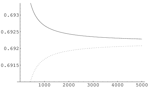
Using these linear time formulas, it is possible to compute and for large values of given a specific functional form for as a function of . A theoretically pleasant, though non-optimal choice, is for even. Recall that can be described by the process whereby the qubits are examined starting from qubit to qubit , and the first zero that is found determines the winner. With , the probability that qubit needs to be examined is , and therefore each qubit determines the outcome with a probability of . The problem with this choice is that Bob’s probability of winning given that qubit needs to be examined keeps oscillating between and numbers greater than . That is why for , Bob has the ability to cheat a lot, whereas Alice is more restricted. With some work, the problem could be fixed by adjusting the values of for and .
The values of and as a function of even for have been plotted in Fig. 4. The upper solid line corresponds to and the lower dotted line to . For odd we would have to use to satisfy the constraint, and this would switch the values of and .
For large , the graphs converge towards , or a bias of . The same behavior occurs with many other reasonable choices for as a function of . We believe that all choices will converge in the limit of to a bias of (or higher for bad choices), but we shall not prove this in the present paper.
VI Summary
We have shown the existence of quantum weak coin-flipping protocols with biases as low as and converging to a number near as . Unfortunately, this appears to be the smallest bias that can be achieved by the protocol described in this paper for any number of rounds.
Many possibilities remain open. The first is that quantum weak coin-flipping with arbitrarily small bias is impossible, and that the optimal bias is either or some number below it. This would be unfortunate, but in the opinion of the author not all that improbable.
Another possibility is that there exists a different family of protocols that produces arbitrarily small bias. In fact, a third possibility is that the protocol presented in this paper has an arbitrarily small bias. This could happen either because some better choice of parameters does produce arbitrarily small bias, or because the upper bounds and are not tight and converge to a different value than the true bias. The last possibility could be eliminated by constructing cheating strategies that achieve biases equal to the upper bound.
Further research will be needed to distinguish these possibilities, and to finally settle the question of whether quantum weak coin-flipping with arbitrarily small bias is possible.
Acknowledgements.
The author would like to thank Ben Toner, Alexei Kitaev and John Preskill for their help. This work was supported in part by the National Science Foundation under grant number EIA-0086038 and by the Department of Energy under grant number DE-FG03-92-ER40701.References
- Blum (1981) M. Blum, Coin flipping by telephone, in Advances in Cryptology: A Report on CRYPTO ’81, edited by A. Gersho (ECE Report No 82-04, Santa Barbara, 1981), pp. 11–15.
- Ambainis (2001) A. Ambainis, A new protocol and lower bounds for quantum coin flipping, in Proceedings on 33rd Annual ACM Symposium on Theory of Computing (ACM, New York, 2001), pp. 134–142, quant-ph/0204022.
- Spekkens and Rudolph (2002a) R. W. Spekkens and T. Rudolph, Degrees of concealment and bindingness in quantum bit commitment protocols, Phys. Rev. A 65, 012310 (2002a), quant-ph/0106019.
- (4) A. Yu. Kitaev, results presented at QIP 2003 (slides and video available from MSRI).
- Ambainis et al. (2003) A. Ambainis, H. Buhrman, Y. Dodis, and H. Roehrig, Multiparty quantum coin flipping (2003), quant-ph/0304112.
- Spekkens and Rudolph (2002b) R. W. Spekkens and T. Rudolph, Quantum protocol for cheat-sensitive weak coin flipping, Phys. Rev. Lett. 89, 227901 (2002b), quant-ph/0202118.
- Kerenidis and Nayak (2004) I. Kerenidis and A. Nayak, Weak coin flipping with small bias, Inf. Process. Lett. 89, 131 (2004).
- Ambainis (2002) A. Ambainis, Lower bound for a class of weak quantum coin flipping protocols (2002), quant-ph/0204063.