Localization of Multi-State Quantum Walk
in One Dimension
Abstract
Particle trapping in multi-state quantum walk on a circle is studied. The time-averaged probability distribution of a particle which moves four different lattice sites according to four internal states is calculated exactly. In contrast with “Hadamard walk” with only two internal states, the particle remains at the initial position with high probability. The time-averaged probability of finding the particle decreases exponentially as distance from a center of a spike. This implies that the particle is trapped in a narrow region. This striking difference is minutely explained from difference between degeneracy of eigenvalues of the time-evolution matrices. The dependence of the particle distribution on initial conditions is also considered.
Keywords:
quantum walk, quantum computer, random walk, localizationPACS
03.67.Lx , 05.40.-a , 89.70.+cE-mail: inui@eng.u-hyogo.ac.jp
E-mail: norio@mathlab.sci.ynu.ac.jp
1 Introduction
The quantum walks attract our attention not only in a fundamental field of quantum mechanics [1] but also in a filed of quantum information [2] (see also recent review with many references [3]). This is because the quantum walks will be achieved on quantum computers [4], and it may be used as a new quantum algorithm.
A classical random walker on a line moves to a nearest left site or a nearest right site randomly at every time step. On the other hand, a quantum walker moves, in superposition, both left and right according to additional degree of freedom called “chirality”. First of all, we describe the Hardamrd walk, which is the most well-known quantum walk. The Hadamard walk is characterized by two parameters. The first is the spatial position and the second is the chirality, which takes values “” and “”. The corresponding Hilbert spaces are and , where is the set of complex numbers. The position space consists of basis states corresponding to the walker located at -th lattice site. Possible experimental implementations of the Hadamard walk have been proposed by a number of authors [4-6]. For example, a quantum walker is an atom and internal states of the atom such as hyperfine structure are used to distinguish the chirality.
Let be a value of wave function at position and time with the chirality . The wave function is changed by superimposing on at ever time step (details are defined in the next section). Assume that a walker exists at the origin in spatial-temporal plane, then we find the walker in the symmetrical Hadamard walk with the same probability at the position 1 or after a single transformation. This behavior is the same as symmetric classical random walk. The primary question in the quantum walk is to determine the probability distribution of the walker after repeating the transformation of wave function. The recent extensive studies made clear mathematical properties of the Hadamard walk. We know that the probability distribution is quite different from that of classical random walk. When the initial wave function is given by and , (symmetric case), we see that double peaks spread in the mutually different direction. Furthermore the standard deviation increases in proportion to time. This means that the quantum walker spreads more quickly than classical random walker, and it is a desirable feature for seeking problems.
Recent studies revealed that there are two distinguishing profiles in modified Hadamard walks on an infinite space. When the walker exists initially at the origin, the one of shapes is concave in a broad way and the other shape is a spike. The spike at the initial time in the symmetrical Hadamard walk sprits two peaks and they move away from the origin as time increases. The probability of finding the walker near the origin decreases and approaches to zero. Thus the probability distribution of the original Hadamard walk belongs to the former. On the other hand, we can always find a walker with high probability near the origin in the later case. We know little about the spiky probability distribution in the later case. The existence of the spikes are already reported in the two-dimensional Grover walk [7,8], one-dimensional quantum walk as many coins [9], but, no probability distributions are calculated explicitly. In this paper we consider quantum walk with four internal states, which is the same as the quantum walk with many coins essentially, and compute analytically the probability distribution. The Hadamard walker described above has two internal quantum states and moves to only nearest neighbor sites, while a walker in “four-state quantum walk” can move beyond nearest neighbor sites by a single transformation.
The rest of this paper is organized as follows. We define multi-state quantum walk generally and show a result obtained by simulation in the next section. In section 3, eigenvalues of the time evolution matrix are exactly calculated and the wavefunction is expressed using those eigenvalues. In section 4, we introduce a time-averaged probability and show that the quantum walker is found with high probability at the initial position. In section 5, a quantum walker with three internal states, in which a walker jumps asymmetrically, is considered and it is shown that localization is not observed.
2 Multi-state quantum walk
We consider a quantum walker with different internal states and moves to different lattice sites according to the internal states. Assume that is an even integer larger than 2. Let . We then define the transformation of -state quantum walk by
| (1) |
where and . This transformation is quite simple, but, it produces rich quantum effects. If the number of internal state is four, we regard the above transformation as the quantum version of the classical random walk in which a walker jumps to each nearest site and next nearest site with the same probability .
Our main conclusion arguing that the particle in -state quantum walk is trapped near the starting point is available for any even except , but in this paper we focus on four-state quantum walk to avoid excessive generality. The transformation with is diffrent from the Hadamard transformation, and the dynamics of -state quantum walk is trivial.
We begin to calculate the probability distribution of the quantum walks on a circle containing sites [10]. We define the probability of finding a walker at position and time by
| (2) |
where “” denotes complex conjugate. To compare the probability distribution between the Hadamard walk and four-state quantum walk, Fig.1 shows the snapshot of probability distribution at starting from an initial wave function:
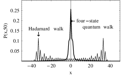
In contrast with the Hadamard walk we clearly find a single spike at the origin in four-state quantum walk. A similar spike has also been observed in two-dimensional quantum walk by simulation [7] and the height of time-averaged probability at the origin is exactly calculated [8]. However, the probability distribution has not been obtained explicitly as a function of the location. For these reason, the main purpose of this paper is to calculate the time-averaged probability distribution of four-state quantum walk and show that the spike in Fig.1 does not disappear even in the thermodynamic limit.
3 Transfer matrix and eigenvalues
The time evolution of the wavefunction of the multi-state quantum walk is determined by transformation Eq. (1) and it is expressed briefly by introducing a time evolution operator satisfying . Since the matrix is unitary, is explicitly given by transforming to a diagonal matrix as a function of the time. Using Fourier transformation it is found that eigenvalues of are calculated from the eigenvalues of the following matrix:
where . Changing the value of from 0 to , we get all eigenvalues of (see details in Ref. [11]). The eigenvalues of are given by
| (16) | |||||
| (17) |
where and for . We stress here that the eigenvalues and are independent of value , put simply, they are strongly degenerative. In fact, the degree of degeneracy for and are and , respectively. Since for , the degree of degeneracy of other eigenvalues is two unless is a multiple of 5. In case of , the classification of eigenvalues is more complicated. Thus we suppose that is odd and is not a multiple of 5 in this paper.
All eigenvalues are now obtained and then the wave function is formally expressed by
| (18) | |||||
where denotes the argument of , and the first and second terms express the contribution of eigenvalue and 1 to the wave function. The coefficients in the above formula are calculated from the eigenvectors of . Let be the eigenvectors corresponding to the eigenvalue of and be the -th element for . We assume additionally is an orthonormal basis. Then the -th element of eigenvectors of the matrix with , which becomes an orthonormal basis is obtained by
| (19) |
where denotes the integer part of . If the walker exists initially at the origin, the coefficient , for example, is expressed by
| (20) |
where , and .
4 Time-averaged probability
In general, the value of wave function at any fixed position does not converge to a constant value. Thus we here define the time-averaged probability of finding the particle at the position and in the internal state in order to show the localization in long time scale as
| (21) |
Noting that for , we have the following equation:
| (22) |
Let us consider time-averaged probability in the limit below. Combining Eqs. (19) and (20), we find that and decrease in the form for large . Therefore the third and fourth terms vanish in the limit of . As a result, time-averaged probability on a circle containing infinite sites is simply given by
| (23) |
Assume that the particle exists at the origin initially. Then the values of for in the right-hand side are determined from only four components of the initial state and they are expressed in the following form:
| (37) |
In this formula, expresses a contribution from the initial state to . If each component of the above matrix in Eq.(37) is exactly obtained, then the time-averaged probability is immediately calculated from Eq.(23) for any initial state.
Let us now calculate . Using the set of eigenvectors of , is given by
| (38) |
We use the following orthonormal eigenvectors corresponding to for and :
where
| (44) |
In case of , since eigenvalues are , and the value degenerate, we use the following eigenvectors which are orthonormal basis
| (45) |
Plugging above eigenvectors into Eq. (19) and carrying out the summation in Eq. (38) we have exactly after a somewhat tedious calculation as follows:
where
| (51) |
The value of , , , and are given by
| (52) |
When the number of size is large, the valuable is almost continuous. Thus the infinite summation is calculated by transforming the summation into the complex integration on the unit circle. The integration is exactly calculated by residue theorem, and and are poles of the function of in Eq. (38), in which is replaced as continuous valuable. Other components are obtained from the following relations:
| (53) |
Although the obtained expression is rather complicated, this formula gives exact values of the time-averaged probability for any initial state and for any position of lattice site.
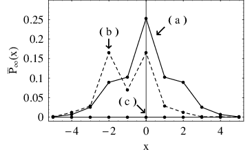
Let us write briefly the initial state by , and consider the time-averaged probability summing over all possible states . Fig.2 shows for three different initial states: (a) symmetrical case , (b) asymmetrical case , and (c) extinction case ,. One clearly finds that the walker is localized near the origin for the case (a) and its shape is almost the same with that in Fig.1. In case of (b), there is a double peak and it shifts to the left. In contrast with (a) and (b), no peaks exist in the case of (c). The probability of finding a walker decreases in inverse proportion to the system size and it converges to zero in the limit of .
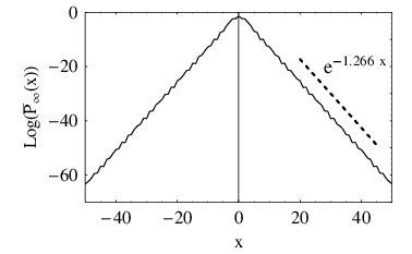
We move our attention to the asymptotic behavior for large . From Eq. (51) each component of the matrices exponentially decreases as increasing the . The values of and are nearly equal to and , respectively, thus the latter contributes largely to . Fig.3 shows as function of with the initial state (a). The slope of inserted line means the exponent of decay is . This exponential decay of the time-averaged probability shows surely that four-state quantum walker localizes near the origin except for special initial states. Very recently similar exponential decay is observed in momentum space of generalized quantum walk by Romanelli et al. [12]. We should remark that only the four-state quantum walk starting from for any real number does not show the localization. This means that the localization is substantially universal property in four-state quantum walk.
5 Three-state quantum walk
We have shown that the four-state quantum walker is fixed near the initial position except special initial conditions. In this section, three-state quantum walk with asymmetrical jump is considered. The time evolution of three-state quantum walk is defined by
In four-state quantum walk, the walker can jump symmetrically to the right and the left. This three-state quantum walker, by contrast, can jump to nearest neighbor sites and a right-hand next-nearest neighbor site, but the walker can not jump to a left-hand next-nearest neighbor site.
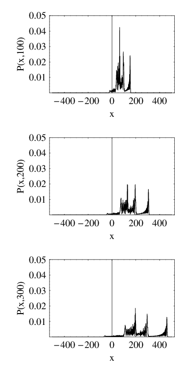
Fig.4 shows snapshots of probability distribution at and 300 starting from the origin with an initial state , . We observe that the several local peaks move to the right and the heights gradually decrease in the prolonged simulation.
The striking difference between four-state and three-state quantum walks is explained from difference in the matrix . The matrix corresponding to three-state quantum walk is given by
The eigenvalues of are exactly obtained. It is easily found that the each degree of degeneracy is independent of the system size. In other words, there is not any eigenvalue corresponding and considered in the previous section. Therefore the height of each peak inevitably approach as to zero in the thermodynamic limit. Consequently, the localization can not be observed in the three-state quantum walk.
6 Summary
The key factor of the localization in the four-state quantum walk is the degeneracy of eigenvalues. If the degree of degeneracy is independent of the dimension of the Hilbert space, the contribution to the time-averaged probability approaches to zero in the limit of . Therefore the existence of eigenvalues whose degree of degeneracy is proportion to the size of the Hilbert space is a necessary condition. This basic condition is also satisfied in the two-dimensional Grover walk. As a result, the walk shows localization [8]. From this criterion we conclude that the Hadamard walk does not exhibit localization. Furthermore we proved that three-state quantum walk with asymmetrical jump does not show the localization.
The time-averaged probability at the initial position in the Grover walk already calculated. However the probability distribution has not been calculated yet. Thus we showed firstly that the time-averaged probability of finding the particle decreases exponentially (not Gaussian) as distance increases from a center of a spike and there are special initial states with which the spike disappears in a one-dimensional quantum walk.
The primary criterion of being localization in probability distribution is only the dependence of degeneracy of eigenvalue on the system size. If the number of the internal state is even, then eigenvalues include and and their degree of degeneracy increase as the system size. Accordingly we can conclude that the multi-state quantum walker with even internal states almost freezes without detailed calculations.
References
- (1) Y. Aharonov, L. Davidovich, and N. Zagury: Phys. Rev. A 48 (1993) 1687.
- (2) A. M. Childs, E. Farhi, and S. Gutmann: Quantum Information Processing 1 (2002) 35.
- (3) J. Kempe: Contemporary Physics 44 (2003) 307.
- (4) B. C. Travaglione and G. J. Milburn: Phys. Rev. A 65 (2002) 032310.
- (5) J. Du, H. Li, X. Xu, M. Shi, J. Wu, X. Zhou, and R. Han: Phys. Rev. A 67, 042316.
- (6) P. L. Knight, E. Roldan, and J. E. Sipe: Optics Communications 227 147.
- (7) B. Tregenna, W. Flanagan, W. Maile, and V. Kendon: New Journal of Physics, 5 (2003), 83.1.
- (8) N. Inui. Y. Konishi, and N. Konno: Phys. Rev. A 69 (2004) 052323.
- (9) T. A. Brun, H. A. Carteret, and A. Ambainis: Phys. Rev. A 67 (2003) 052317.
- (10) D. Aharonov, A. Ambainis, J. Kempe, and U. V. Vazirani: Proc. of the 33rd Annual ACM Symposium on Theory of Computing, 272 (2001) 50.
- (11) M. Bednarska, A. Grudka, P. Kurzynski T. Luczak, and A. Wojcik: Phys. Lett. A 317 (2004) 21.
- (12) A. Romanelli, A Auyuanet, R. Siri, G. Abal, and R. Donangelo: quant-ph/0408183.