Distributed quantum computing: A distributed Shor algorithm

Anocha Yimsiriwattana and Samuel J. Lomonaco Jr.^a ^aDept. of Computer Sci. and Electrical Eng University of Maryland Baltimore County
1000 Hilltop Circle Baltimore MD USA 25000

Abstract

We present a distributed implementation of Shor’s quantum factoring algorithm on a distributed quantum network model. This model provides a means for small capacity quantum computers to work together in such a way as to simulate a large capacity quantum computer. In this paper, entanglement is used as a resource for implementing non-local operations between two or more quantum computers. These non-local operations are used to implement a distributed factoring circuit with polynomially many gates. This distributed version of Shor’s algorithm requires an additional overhead of $O((\log N)^{2})$ communication complexity, where $N$ denotes the integer to be factored.

keywords

Shor’s algorithm, factoring algorithm, distributed quantum algorithms, quantum circuit.

^†^†authorinfo: Further author information: (Send correspondence to Anocha Yimsiriwattana)
Anocha Yimsiriwattana: E-mail: ayimsi1@umbc.edu, URL: http:/userpages.umbc.edu/~ayimsi1
Samuel J. Lomonaco Jr.: E-mail: lomonaco@umbc.edu, URL: http:/www.cs.umbc.edu/~lomonaco

1 Introduction

To utilize the full power of quantum computation, one needs a scalable quantum computer with a sufficient number of qubits. Unfortunately, the first practical quantum computers are likely to have only small qubit capacity. One way to overcome this difficulty is by using the distributed computing paradigm. By a distributed quantum computer, we mean a network of limited capacity quantum computers connected via classical and quantum channels. Quantum entangled states, in particular generalized GHZ states, provide an effective way of implementing non-local operations, such as, non-local CNOTs and teleportation [1, 2].

We use distributed quantum computing techniques to construct a distributed quantum circuit for the Shor factoring algorithm. Let $n=\log N$ , where $N$ is the number to be factored. The gate complexity of this particular distributed implementation of Shor’s algorithm is $O(n^{3})$ with $O(n^{2})$ communication overhead.¹¹ 1 Shor’s factoring algorithm is of gate complexity $O(n^{2}\log n\log\log n)$ and space complexity $O(n\log n\log\log n)$ .

In section 2, the general principles of distributed quantum computing are outlined, and two primitive distributed computing operators, cat-entangler and cat-disentangler, are introduced. We use these two primitive operators to implement non-local operations, such as non-local CNOTs and teleportation. Then we discuss how to share the cost of implementing a non-local controlled $U$ , where $U$ can be decomposed into a number of gates. The section ends with an distributed implementation of the Fourier transform.

In section 3, we give a detailed description of an implementation of Shor’s non-distributed factoring algorithm. This implementation is based on the phase estimation and order finding algorithms. We discuss in detail how to implement “modular exponentiation,” which implementation will be used later in this paper as a blueprint for creating a distributed quantum algorithm.

In section 4, we implement a distributed factoring algorithm by partitioning the qubits into groups in such a way that each group fits on one of the computers making up the network. We then proceed to replace controlled gates with non-local controlled gates whenever necessary.

2 Distributed quantum computing

By a distributed quantum computer (DQC), we mean a network of limited capacity quantum computers connected via classical and quantum channels. Each computer (or node) possesses a quantum register that can hold only a fixed limited number of qubits. Each node also possesses a small fixed number of channel qubits which can be sent back and forth over the network. Each register qubit can freely interact with any other qubit within the same register. Each such qubit can also freely interact with channel qubits that are in the same computer. In particular, each such qubit can interact with other qubits on a remote computer by two methods: 1) The qubit can interact via non-local operations, or 2) The qubit can be teleported or physically transported to a remote computer in order to locally interact with a qubit on that remote computer.

Indeed, distributed quantum computing can be implemented by only teleporting or physically transporting qubits back and forth. However, a more efficient implementation of DQC has been proposed by Eisert et al [1] using non-local CNOT gates. Since the controlled-NOT gate together with all one-qubit gates is universal set of gates [3], a distributed implementation of any unitary transformation reduces to the implementation of non-local CNOT gates. Eisert et al also prove that one shared entangled pair and two classical bits are necessary and sufficient to implement a non-local CNOT gate.

Yimsiriwattana and Lomonaco [2] have identified two primitive operations, cat-entangler and cat-disentangler, which can be used to implement non-local operations, e.g., non-local CNOTs, non-local controlled gates, and teleportation. Figure 1 illustrates cat-entangler and cat-disentangler operations.

Refer to caption — Figure 1: The cat-entangler and cat-disentangler operations for a 5-qubit system are shown in figure 1-A and figure 1-B, respectively. A dotted-line represents a measurement result, which is classical and is used to control $X$ gates. The $Z$ gate in circuit 1-B is controlled by the exclusive-or $(\oplus)$ of the three classical bits resulting from the measurement of qubits three to five. A qubit is reset to $|{0}\rangle$ by a control- $X$ gate. This control- $X$ gate is controlled by a classical bit arising from the measurement on the qubit.

For the implementation of a non-local CNOT gate, an entangled pair must first be established between two computers. Then, the cat-entangler is used to transform a control qubit $\alpha|{0}\rangle+\beta|{1}\rangle$ and an entangled pair ${{1\over\sqrt{2}}(|{00}\rangle+|{11}\rangle)}$ into the state $\alpha|{00}\rangle+\beta|{11}\rangle$ , called a “cat-like” state. This state permits two computers to share the control qubit. As a result, each computer now can use a qubit shared within the cat-like state as a local control qubit.

After completion of the control operation, the cat-disentangler is then applied to disentangle and restore the control qubit from the cat-like state. Finally, channel qubits are reset by using the classical information resulting from measurement to control $X$ gates. In this way, channel qubits can be reused and entangled pairs can be re-established. A non-local CNOT circuit is illustrated in figure 2-A.

To teleport an unknown qubit from computer A to B, we begin by establishing an entangled pair between two computers. Then, we apply the cat-entangler operation to create a cat-like state from an unknown qubit and the entangled pair. After that, we apply a cat-disentangler operation to disentangle and restore the unknown qubit from the cat-like state into the computer B. Finally, we reset the channel qubits by swapping the unknown qubit with $|{0}\rangle$ . The teleportation circuit is shown in figure 2-B.

Because a cat-like state permits two computers to share a control qubit, the cost of implementing a non-local controlled $U$ , where $U$ is a unitary transformation composed of a number of basic gates, can be shared among these basic gates.

For example, let us assume that a unitary transformation has the form $U=U_{1}\cdot U_{2}\cdot U_{3}$ , where $U_{3}=CNOT$ . Since the control qubit is reused, each non-locally controlled $U_{i}$ gate can be implemented using asymptotically only ${1\over{3}}$ entangled pair and $2\over 3$ classical bit, as demonstrated in figure 3.

Before the execution of a non-local operation, an entangled pair must first be established between channel computers. If each machine possesses two channel qubits, then two entangled pairs can be established by sending two qubits. To do so, each computer begins by entangling its own channel qubits, then exchanging one qubit of the pair with the other computer. As a result, one entangled pair is established at the asymptotically cost of sending one qubit. To refresh the entanglement, the procedure is simply repeated after the channel qubits are reset to the state $|{0}\rangle$ .

2.1 Distributed quantum Fourier transform

The quantum Fourier transform is a unitary transformation defined on standard basis states as follows,

|{j}\rangle\rightarrow{1\over{\sqrt{2^{n}}}}\sum_{k=0}^{2^{n}-1}e^{2\pi\imath jk/2^{n}}|{k}\rangle,

(1)

where $n$ is the number of qubits.

An efficient circuit for the quantum Fourier transformation can be found in Nielsen and Chuang’s book [9] and also in Cleve et al. paper [5]. We implement a distributed version of the Fourier transformation by replacing a controlled $R_{k}$ with non-local controlled $R_{k}$ , when necessary. The distributed swap gate can be implemented by teleporting qubits back and forth between two computers. An implementation of the distributed Fourier transformation of $4$ qubits is shown in figure 4, where the gate $R_{k}$ is defined as:

\displaystyle R_{k}=\left(\begin{array}[]{cc}{1}&{0}\\ {0}&{e^{2\pi\imath/2^{k}}}\end{array}\right),

for $k\in\left\{{2,3,\ldots}\right\}$ .

For a more detailed discussion on distributed quantum computing, please consult Yimsiriwattana and Lomonaco [2].

3 The quantum factoring algorithm

The prime factorization problem is defined as follows: Given a composite odd positive number $N$ , find its prime factors [6].

It is well known that factoring a composite number $N$ reduces to the task of choosing a random integer $a$ relatively prime to $N$ , and then determining its multiplicative order $r$ modulo $N$ , i.e., to find the smallest positive integer $r$ such that $a^{r}=1\ (mod\ N)$ . This problem is known as the “order finding problem.”

Cleve et al [5] have shown that the order finding problem reduces to the phase estimation problem, a problem which can be solved efficiently by a quantum computer. We briefly review these problems in this section.

3.1 Phase Estimation Algorithm

The phase estimation problem is defined as follows: Let $U$ be an $n$ -qubit unitary transformation having eigenvalues

\lambda_{0}=e^{2\pi\imath\theta_{0}},\ldots,\lambda_{2^{n}-1}=e^{2\pi\imath\theta_{2^{n}-1}}

with corresponding eigenkets

|{\psi_{0}}\rangle,\ldots,|{\psi_{2^{n}-1}}\rangle

where $0\leq\theta_{k}<1$ . Given one of the eigenket $|{\psi_{t}}\rangle$ , estimates the value of $\theta_{t}$ .

Cleve et al solve this problem as follows: Construct two quantum registers, the first an $m$ -qubit register, and the second an $n$ -qubit register. Then construct a unitary transformation $c_{m}(U)$ which acts on both registers as follows:

c_{m}(U):|{k}\rangle|{\psi}\rangle\rightarrow|{k}\rangle U^{k}|{\psi}\rangle

(5)

where $|{k}\rangle$ and $|{\psi}\rangle$ denotes respectively the state of the first and second register. The phase estimation algorithm can be described as follows:

Phase Estimation Algorithm:
Input: $U$ and $|{\psi_{t}}\rangle$ , Output: An estimate of $\theta_{t}$ .
Note: $|{r_{1}}\rangle$ ( $|{r_{2}}\rangle$ ) is the state of the first register (second register, respectively).
(1) Let $|{r_{1}}\rangle|{r_{2}}\rangle=|{0}\rangle|{\psi_{t}}\rangle$ .
(2) $|{r_{1}}\rangle|{r_{2}}\rangle=(H^{\otimes m}\otimes I)|{r_{1}}\rangle|{r_{2}}\rangle$ .
(3) $|{r_{1}}\rangle|{r_{2}}\rangle=c_{m}(U)|{r_{1}}\rangle|{r_{2}}\rangle$ .
(4) $|{r_{1}}\rangle|{r_{2}}\rangle=(QFT^{-1}\otimes I)|{r_{1}}\rangle|{r_{2}}\rangle$ .
(5) $j$ = the result of measuring $|{r_{1}}\rangle$
(6) Output $j/2^{m}$ .

Step (1) is an initialization of the registers into the state $|{0}\rangle|{\psi_{t}}\rangle$ with input $|{\psi_{t}}\rangle$ . Step (2) applies the Hadamard transformation to the first register, leaving the registers in the state

|{r_{1}}\rangle|{r_{2}}\rangle={{1\over\sqrt{2^{m}}}}\sum_{k=0}^{2^{m}-1}|{k}\rangle|{\psi_{t}}\rangle.

(6)

As a result of applying $c_{m}(U)$ in step (3), the registers are in the state

\displaystyle|{r_{1}}\rangle|{r_{2}}\rangle

\displaystyle=

\displaystyle{{1\over\sqrt{2^{m}}}}\sum_{k=0}^{2^{m}-1}e^{2\pi\imath k\theta_{t}}|{k}\rangle|{\psi_{t}}\rangle.

(7)

To understand the workings of step (4), let us assume that $\theta_{t}=j/2^{m}$ , for some $j\in\left\{{0,\ldots,2^{m}-1}\right\}$ . Therefore, the equation (7) can be rewritten as:

|{r_{1}}\rangle|{r_{2}}\rangle={{1\over\sqrt{2^{m}}}}\sum_{k=0}^{2^{m}-1}e^{2\pi\imath kj/2^{m}}|{k}\rangle|{\psi_{t}}\rangle.

(8)

By applying the inverse quantum Fourier transform in step (4), the registers are in the state

|{r_{1}}\rangle|{r_{2}}\rangle=|{j}\rangle|{\psi_{t}}\rangle.

(9)

By making a measurement on the first register in step (5), we obtain $j$ , where $\theta_{t}=j/2^{m}$ .

In general, $\theta_{t}$ may not be of the form of $j/2^{m}$ . However, the result of applying the inverse QFT in step (4) results in $j/2^{m}$ being the best $m$ -bit estimation of $\theta_{t}$ with a probability of at least $4/\pi^{2}$ . For more details, please consult Cleve et al [5]. A quantum circuit of the phase estimation algorithm is shown in figure 5.

3.2 Order Finding Algorithm

The order finding problem is defined as follows: Given a positive integer $N$ and an integer $a$ relatively prime to $N$ , find the smallest positive integer $r$ such that

a^{r}=1\ (mod\ N).

(10)

First of all, we want a unitary transformation to use in the phase estimation algorithm. We call that unitary transformation $M_{a}$ , which is defined as follows:

M_{a}:|{x}\rangle\rightarrow|{ax\ (mod\ N)}\rangle,

(11)

where $|{x}\rangle$ is an $n$ -qubit register (the second register). Let $\omega=e^{2\pi\imath\over r}$ , and for each $k\in\left\{{0,\ldots,2^{n}-1}\right\}$ , define

|{\psi_{t}}\rangle={1\over\sqrt{r}}\sum_{s=0}^{r-1}\omega^{-st}|{a^{s}}\rangle.

(12)

Then, for each $t$ , $M_{a}|{\psi_{t}}\rangle=\omega^{t}|{\psi_{t}}\rangle.$ In other words, $\omega^{t}$ is an eigenvalue of $M_{a}$ with respect to eigenvector $|{\psi_{t}}\rangle$ . Furthermore, $\theta_{t}\approx t/r$ , for each $t$ . Therefore, if we have given an eigenvector $|{\psi_{1}}\rangle$ , and we know how to construct $c_{m}(M_{a})$ , then we can find $r$ (which is the period of $a$ ) by using the phase estimation algorithm.

Unfortunately, it is not trivial to construct $|{\psi_{t}}\rangle$ for every $t$ . Instead of using $|{\psi_{t}}\rangle$ , we use $|{1}\rangle$ which is effectively equivalent to selecting $|{\psi_{t}}\rangle$ , where $t$ is randomly selected from $\left\{{0,\ldots,r-1}\right\}$ . Then, we use the phase estimation algorithm to compute the value of $j/2^{m}$ which is the best $m$ -bit estimate value of $t/r$ . We extract the value of $t/r$ by using the continued fraction algorithm. If $t$ and $r$ are relatively prime, then we get $r$ , which is the period of $a$ . The output $r$ of the phase estimation algorithm can be tested by checking that $a^{r}=1(modN)$ . If $r$ is not the period of $a$ , then we can re-execute this algorithm until $t$ is coprime to $r$ , which occurs with high probability in $O(\log\log N)$ rounds [5].

In the next section, we describe an implementation of $c_{m}(U)$ . This calculation is equivalent to the calculation that Shor uses in his factoring algorithm, known as “modular exponentiation.” Another detailed implementation of the modular exponentiation can be found in Beckman et al [7].

3.3 An implementation of modular exponentiation

To complete the implementation of the order finding algorithm, we need to construct the unitary transformation $c_{m}(M_{a})$ . We accomplish this by using the method of repeated squaring.

Let $k_{m-1}k_{m-2}\ldots k_{1}k_{0}$ , be the binary expansion of the contents of the first register, $|{k}\rangle$ . It now follows that

M_{a}^{k}=\prod_{i=0}^{m-1}M_{a}^{k_{i}2^{i}}=\prod_{i=0}^{m-1}(M_{a}^{2^{i}})^{k_{i}}.

(13)

Then, for each $i$ , we can implement the term $(M_{a}^{2^{i}})^{k_{i}}$ as a controlled $M_{a}^{2^{i}}$ , where the control qubit is $|{k_{i}}\rangle$ .

Please note that $a$ is a constant integer, and that $M_{a}^{2^{i}}=M_{a^{2^{i}}}$ for all $0\leq i<m$ . Therefore, we can precompute the value of $a^{2^{i}}$ by classical computers. Then we can apply the same technique used to implement $M_{a}$ , to implement $M_{a^{2^{i}}}$ . Figure 6 shows an implementation of $c_{m}(M_{a})$ .

3.3.1 Reusing ancillary qubits

For a given polynomial-time function $f$ , we can construct a unitary transformation $F$ which maps $|{x}\rangle|{0}\rangle$ to $|{x}\rangle|{f(x)}\rangle$ . However, the complete definition of $F$ also includes ancillary qubits which contain information necessary for $F$ to be reversed. Let $g$ be a function that computes the additional information, called “garbage”. The complete definition of $F$ is,

F:|{x}\rangle|{0}\rangle|{0}\rangle\rightarrow|{x}\rangle|{f(x)}\rangle|{g(x)}\rangle,

(14)

The garbage needs to be reset, or erased, to state $|{0}\rangle$ before we make a measurement. Otherwise, the result of the measurement could be affected by the garbage. To erase the garbage, Shor uses Bennett’s technique which we review in this section.

First we compute $F(x)$ . Once we have the output $|{f(x)}\rangle$ , we copy $|{f(x)}\rangle$ into the extra register which has been preset to state $|{0}\rangle$ . Then we erase the output and the garbage of $F$ by reverse computing $F(x)$ . In particular, this procedure is described as follows:

$\displaystyle\|{x}\rangle\|{0}\rangle\|{0}\rangle\|{0}\rangle$	$\displaystyle\stackrel{{\scriptstyle F}}{{\Longrightarrow}}$	$\displaystyle\|{x}\rangle\|{f(x)}\rangle\|{g(x)}\rangle\|{0}\rangle$
	$\displaystyle\stackrel{{\scriptstyle\mbox{COPY}}}{{\Longrightarrow}}$	$\displaystyle\|{x}\rangle\|{f(x)}\rangle\|{g(x)}\rangle\|{f(x)}\rangle$
	$\displaystyle\stackrel{{\scriptstyle F^{r}}}{{\Longrightarrow}}$	$\displaystyle\|{x}\rangle\|{0}\rangle\|{0}\rangle\|{f(x)}\rangle,$

where $F^{r}$ is the reverse computation of $F$ . We copy $|{f(x)}\rangle$ to the extra register bit by bit by applying a $CNOT$ gate on each qubit. We define $XF=F^{r}\cdot\mbox{COPY}\cdot F$ .

If $f$ is a polynomial-time invertible function, we can create a unitary transformation $OF$ which overwrites an input $|{x}\rangle$ with the output $|{f(x)}\rangle$ . We start from the construction of a unitary transformation $FI$ as follows:

FI:|{x}\rangle|{0}\rangle\rightarrow|{x}\rangle|{f^{-1}(x)}\rangle,

(15)

where $f^{-1}$ is a polynomial-time inverse function of $f$ . The transformation $FI$ may generate garbage, but it can be erased by using the technique mentioned above. Finally, we implement $OF$ as follows:

$\displaystyle\|{x}\rangle\|{0}\rangle$	$\displaystyle\stackrel{{\scriptstyle F}}{{\Longrightarrow}}$	$\displaystyle\|{x}\rangle\|{f(x)}\rangle$
	$\displaystyle\stackrel{{\scriptstyle\mbox{SWAP}}}{{\Longrightarrow}}$	$\displaystyle\|{f(x)}\rangle\|{x}\rangle$
	$\displaystyle\stackrel{{\scriptstyle FI^{r}}}{{\Longrightarrow}}$	$\displaystyle\|{f(x)}\rangle\|{0}\rangle,$

where $FI^{r}$ is the reverse computation of $FI$ . The SWAP is a swap gate that swaps the content of the input and the output registers.

3.3.2 Binary adders

We continue our construction of $M_{a}$ by first implementing “binary adders.” There are two types of binary adders, “binary full adder” and “binary half adder,” denoted by $\mbox{BFA}_{a}$ and $\mbox{BHA}_{a}$ , respectively. The $\mbox{BFA}_{a}$ and $\mbox{BHA}_{a}$ are defined as follows:

\displaystyle\mbox{BFA}_{a}:|{c}\rangle|{b}\rangle|{0}\rangle\rightarrow|{a\oplus b\oplus c}\rangle|{b}\rangle|{c^{\prime}}\rangle

\displaystyle\mbox{BHA}_{a}:|{c}\rangle|{b}\rangle\rightarrow|{a\oplus b\oplus c}\rangle|{b}\rangle,

(16)

where $a$ is a classical bit, and $|{c}\rangle$ and $|{c^{\prime}}\rangle$ are input and output carries, respectively. The circuits for $\mbox{BFA}_{a}$ and $\mbox{BHA}_{a}$ are shown in figure 7.

The dotted-line represents a classical bit $a$ which is used to control the quantum gates. If the classical bit is $0$ , the quantum gate is not applied. If the classical bit is $1$ , then the quantum gate is applied. The binary full adder adds a classical bit $a$ to the carry $|{c}\rangle$ first, then adds a qubit $|{b}\rangle$ to the sum. Because the carry is not computed by $\mbox{BHA}_{a}$ , we remove two gates (the first gate, and the Toffoli gate) from $\mbox{BFA}_{a}$ in order to implement $\mbox{BHA}_{a}$ .

3.3.3 An $n$ -qubit adder

For each classical $n$ -bit integer $a$ , an $n$ -qubit full adder $\mbox{FA}_{a}$ is the unitary transformation defined by

\mbox{FA}_{a}:|{b}\rangle|{0}\rangle|{c}\rangle\rightarrow|{b}\rangle|{s}\rangle|{c^{\prime}}\rangle

(17)

where $|{s}\rangle$ is an $n$ -qubit register, $s=a+b+c\ (mod\ 2^{n})$ , and $c$ and $c^{\prime}$ are an input and output carries, respectively. A quantum circuit for $\mbox{FA}_{a}$ is shown in figure 8, where $a_{n-1}\cdots a_{1}a_{0}$ , $b_{n-1}\cdots b_{1}b_{0}$ , and $c_{n-1}\cdots c_{1}c_{0}$ are $n$ -bit binary representations of $a,b$ and $c$ , respectively.

We replace the last $\mbox{BFA}_{a_{n-1}}$ with a $\mbox{BHA}_{a_{n-1}}$ to construct $HA_{a}$ . As a result, we need only $n-1$ input ancillary qubits with initial state $|{0}\rangle$ to implement $\mbox{HA}_{a}$ . By including an input carry qubit $|{c}\rangle$ , the $\mbox{HA}_{a}$ is a $2n$ -qubit unitary transformation.

An $n$ -qubit adder modulo $N$

We use $\mbox{FA}_{a}$ and $\mbox{HA}_{a}$ to implement the $n$ -qubit adder modulo $N$ , $(\mbox{AN}_{a})$ . We observe that if $a+b<N$ , then $a+b\ (mod\ N)=a+b\ (mod\ 2^{n})$ ; otherwise $a+b\ (mod\ N)=a+b+2^{n}-N\ (mod\ 2^{n})$ . We implement $\mbox{AN}_{a}$ as follows: First we compute the sum of $|{b}\rangle$ with a classical number $a+2^{n}-N$ in modulo $2^{n}$ . If the carry is not set, then we subtract $2^{n}-N$ from the sum. Hence, we have a transformation $\mbox{AN}_{a}$ , given by

\mbox{AN}_{a}:|{b}\rangle|{0}\rangle|{0}\rangle|{0}\rangle\rightarrow|{b}\rangle|{s}\rangle|{c}\rangle|{a+b\ (mod\ N)}\rangle.

(18)

where $s=b+a+2^{n}-N\ (mod\ 2^{n})$ , and $c$ is the carry. The circuit that implements $\mbox{AN}_{a}$ is shown in figure 9.

We use the technique described in section 3.3.1 to reset $|{s}\rangle$ and $|{c}\rangle$ back to state $|{0}\rangle$ . As a result, we obtain a transformation $\mbox{XAN}_{a}=\mbox{AN}_{a}^{r}\cdot\mbox{COPY}\cdot\mbox{AN}_{a}$ which acts as follows:

\mbox{XAN}_{a}:|{b}\rangle|{0}\rangle|{0}\rangle|{0}\rangle|{0}\rangle\rightarrow|{b}\rangle|{0}\rangle|{0}\rangle|{0}\rangle|{a+b\ (mod\ N)}\rangle.

(19)

In other words, $\mbox{XAN}_{a}$ is a $2n$ -qubit transformation (with $2n+1$ ancillary qubits) which sends $|{b}\rangle|{0}\rangle$ to $|{b}\rangle|{a+b\ (mod\ N)}\rangle$ . The wiring diagram for $\mbox{XAN}_{a}$ is shown in figure 10.

Because the inverse transformation of $\mbox{XAN}_{a}$ is $\mbox{XAN}_{-a}$ , the input of $\mbox{XAN}_{a}$ can be overwritten by the output of $\mbox{XAN}_{a}$ by using the technique described in section 3.3.1. We now define the adder $A_{a}$ as follows:

A_{a}=\mbox{XAN}_{-a}^{r}\cdot\mbox{SWAP}\cdot\mbox{XAN}_{a}.

(20)

As a result, the transformation $A_{a}$ is an $n$ -qubit transformation (with $3n+1$ ancillary qubits) which maps $|{b}\rangle$ to $|{a+b\ (mod\ N)}\rangle$ .

3.3.4 An $n$ -qubit multiplier

Now we are ready to describe the construction of $M_{a}$ , which maps $|{x}\rangle$ to $|{ax}\rangle$ , where $x\in\mathbb{Z}_{N}$ . We define an $2n$ -qubit unitary transformation $MF_{a}$ as follows:

MF_{a}:|{x}\rangle|{0}\rangle\rightarrow|{x}\rangle|{ax(mod\ N)}\rangle.

(21)

Assuming $x_{n-1}\ldots x_{1}x_{0}$ is the binary representation of $x$ , we have

ax=\sum_{i=0}^{n-1}ax_{i}2^{i}.

(22)

For each $0\leq i<n$ , the term $ax_{i}2^{i}$ can be implemented by the control- $A_{a2^{i}}$ , where $|{x_{i}}\rangle$ is a control qubit, and

A_{a2^{i}}:|{b}\rangle\rightarrow|{b+a2^{i}\ (mod\ N)}\rangle.

(23)

Since for each $i$ , $a2^{i}$ is constant, we can compute each $a2^{i}$ by using a classical computer. Then we use the result and the same technique for implementing $A_{a}$ , as described in section 3.3.3, to construct $A_{a2^{i}}$ . Therefore, the transformation $MF_{a}$ can be implemented using the method of repeated squaring with a circuit similar to the circuit shown in figure 6. Hence, $MF_{a}$ is a $2n$ -qubit transformation sending $|{x}\rangle|{0}\rangle$ to $|{x}\rangle|{ax}\rangle$ , using of $3n+1$ ancillary qubits.

Finally, with the overwriting output technique described in section 3.3.1, the transformation $M_{a}$ can be implemented as $M_{a}=MF_{a^{-1}}\cdot\mbox{SWAP}\cdot MF_{a}$ . (Note that, because $a$ and $N$ are relatively prime, $a^{-1}$ always exists in $\mathbb{Z}_{N}$ .) In other words, $M_{a}$ is an $n$ -qubit transformation with $4n+1$ ancillary qubits. Thus, the so constructed $M_{a}$ can be plugged into the transformation $c_{m}(M_{a})$ , as described earlier in section 3.3.

3.4 Complexity analysis

We analyze the complexity of our implementation of Shor’s algorithm for two parameters,i.e., the number of gates and the number of qubits.

Gate complexity

To count the number of gates, we define a function $G(F)$ to be the number of gates used to implement the transformation $F$ . We recursively compute the number of gates as follows:

$\displaystyle G(SHOR)$	$\displaystyle=$	$\displaystyle G(H^{\otimes m}+G(c_{m}(M_{a}))+G(QFT^{-1})$
$\displaystyle G(c_{m}(M_{a}))$	$\displaystyle=$	$\displaystyle m\cdot G(M_{a})$
$\displaystyle G(M_{a})$	$\displaystyle=$	$\displaystyle n\cdot G(A_{a})$
$\displaystyle G(A_{a})$	$\displaystyle=$	$\displaystyle 2\cdot G(\mbox{XAN}_{a})+G(\mbox{SWAP})$
$\displaystyle G(\mbox{XAN}_{a})$	$\displaystyle=$	$\displaystyle 2\cdot G(\mbox{AN}_{a})+G(\mbox{COPY})$
$\displaystyle G(\mbox{AN}_{a})$	$\displaystyle=$	$\displaystyle G(\mbox{FA}_{a})+G(\mbox{HA}_{a})+1$
$\displaystyle G(\mbox{FA}_{a})$	$\displaystyle=$	$\displaystyle n\cdot G(\mbox{BFA})=4n$
$\displaystyle G(\mbox{HA}_{a})$	$\displaystyle=$	$\displaystyle(n-1)\cdot G(\mbox{BFA})+G(\mbox{BHA})=4n-2$

Since $G(H^{\otimes m})=m$ , $G(QFT^{-1})=m(m+1)/2=O(m^{2})$ , and $G(c_{m}(M_{a}))=70mn^{2}-6mn=O(mn^{2})$ , it follows that the gate complexity of this implementation is $O(mn^{2})$ . In general, $m=2n$ . Therefore, the complexity is $O(n^{3})$ .

However, we count a control-gate with multiple control-qubits as one gate. In fact, a control gate with multiple control qubit can be broken down into a sequence of Toffoli gates using the techniques described by Beranco et al [8]. Moreover, the number of needed Toffoli gates grows exponentially with respect to the number of control qubits in the control-gate. Fortunately, the number of control qubits in the Shor’s algorithm is at most $5$ : One control qubit for $c_{m}(M_{a})$ , one control qubit for $M_{a}$ , one control qubit for control- $\mbox{FA}_{a}$ in the implementation of $\mbox{AN}_{a}$ , and two control qubits in the implementation of $\mbox{FA}_{a}$ . Moreover, the number of control qubits does not depend on the input number $N$ . Therefore, there is constant overhead from breaking down a control gate with multiple control qubits into a sequence of Toffoli gates. This overhead does not have affect the gate complexity.

Space complexity

First of all, $\mbox{XAN}_{a}$ is a $2n$ -qubit transformation with $2n+1$ ancillary qubits. So, we need $n$ qubits to control the transformation $A_{a}$ in the implementation of $M_{a}$ , and $m$ more qubits to control the transformation $M_{a}$ in the implementation of $c_{m}(M_{a})$ . Therefore, the number of qubits needed in this implementation is $5n+m+1$ .

4 Distributed quantum factoring algorithm

We implement a distributed quantum factoring algorithm as briefly described as follows: First, we partition $5n+m+1$ qubits into groups in such a way that each group fits on one of the quantum computers making up a network. Then, we implement a distributed quantum factoring algorithm on this quantum network by replacing a control gate with a non-local control gate, whenever necessary.

In this paper, we will describe a distributed quantum factoring algorithm to factor a number $N$ within specific parameters. We assume that we have a network of $(n+c)$ -qubit quantum computers, where $n=\log N$ . The $c$ extra qubits for each computer can be used as either channel qubits or ancillary qubits. We will show that $c$ is a constant which does not depend on the input number $N$ . To be more specific, we choose $m=2n$ . Therefore, the number of qubits needed in this implementation is $7n+1$ qubits. Although, this particular implementation is specific to certain parameters, its implementation can easily be generalized.

First we divide the control register of $c_{m}(M_{a})$ , $|{k}\rangle$ , into two $n$ -qubits groups. Then we place these two groups on two different computers. Each qubit $|{k_{i}}\rangle$ of these two groups remotely controls the transformation $M_{a}^{2^{i}}$ .

Another computer is assigned to hold the control register of $MF_{a}$ , i.e., $|{x}\rangle$ . Each qubit $|{x_{j}}\rangle$ remotely controls the transformation $A_{a}$ .

Next, we implement the transformation $\mbox{XAN}_{a}$ , which is a component of $\mbox{AN}_{a}$ . The transformation $\mbox{XAN}_{a}$ has two registers, one $n$ -qubit input register $|{b}\rangle$ , and one $n$ -qubit output register $|{a+b}\rangle$ . However, $\mbox{XAN}_{a}$ also requires $2n+1$ ancillary qubits, i.e., one carry bit, $n$ qubits for the intermediate sum $|{s}\rangle$ , and $n$ qubits for the intermediate output register $|{a+b}\rangle$ . Therefore, it takes four computers to compute $\mbox{XAN}_{a}$ . Each computer computes $1/4$ of each register, as shown in figure 11. Each computer holds $n/4$ qubits from the input registers $|{b}\rangle$ , $n/4$ qubits from the intermediate sum register $|{s}\rangle$ , $n/4$ qubits from the intermediate output register, and $n/4$ qubits from the output register $|{a+b}\rangle$ (represented by thick lines). Each computer also has two extra carries qubits, which are used in computing of FA and $\mbox{FA}^{\prime}$ .

The first four FA transformations compute $\mbox{FA}_{a+2^{n}-N}$ with the input carry $|{c}\rangle=|{0}\rangle$ . These FAs are remotely controlled by two control qubits, one from the register $|{k}\rangle$ , and the other from the register $|{x}\rangle$ . A distributed control FA with two control qubits is implemented by distributing two control qubits onto the computer that holds the target qubits, and then implementing the double control locally, as shown in figure 12. After completing each FA computation, the output carry bit is teleported to the next FA on another computer. The teleportations are represented by arrow lines.

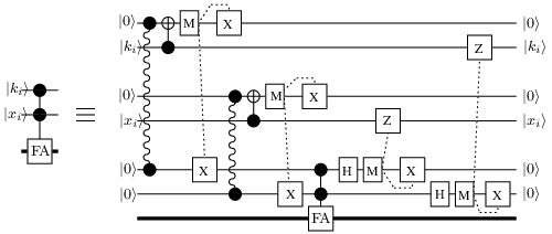
The transformation $\mbox{HA}_{-(2^{n}-N)}$ is computed by the next three full adders $\mbox{FA}^{\prime}$ , and a half adder HA. The integer $-(2^{n}-N)$ is precomputed by a classical computer, and then used to implement $\mbox{FA}^{\prime}$ and HA. Similarly, the carry qubit is teleported from one computer to another. The last carry qubit is teleported into the first qubit of the intermediate output register $|{(a+b)_{3n/4\cdots n-1}}\rangle$ .

Each $\mbox{FA}^{\prime}$ and the single HA are each controlled by three qubits: One from the first register $|{k}\rangle$ , one from the register $|{x}\rangle$ , and the last from the output carry bit of $\mbox{FA}_{a+a^{n}-N}$ . A non-local three-control gate can implemented by distributing all three-control qubits onto the target computer, and locally implementing the control gate with three control qubits.

The COPY transformation is a bitwise copy implemented in terms of CNOT gates. Because each computer possesses $n/4$ of intermediate output register and the final output register itself, the distributed COPY can be easily implement by locally applying CNOT gates, as shown in figure 11. However, COPY still needs to be remotely controlled by two qubits from register $|{k}\rangle$ and register $|{x}\rangle$ .

Similarly, each machine possesses $n/4$ qubits of both input register and output register. The distributed SWAP can be locally implement on each machine, remotely controlled by two qubits from register $|{k}\rangle$ and register $|{x}\rangle$ .

The number of extra qubits

The number of extra qubits $c$ depends on two factors: The number of channel qubits, and the number of extra carry qubits needed in the implementation. The number of channel qubits depends on how many non-local control qubits are needed. In this implementation, at most three non-local control qubits are implemented. Therefore, at most $3$ channel qubits are required at one time. Furthermore, there are only two extra carry qubits (one carry qubit for transformation FA and another carry qubit for transformation $\mbox{FA}^{\prime}$ ) needed in this implementation. Therefore, $c=5$ , and does not depend on the input $N$ .

4.1 Communication complexity

By communication complexity, we means the number of entangled pairs needed to be established, and the number of classical bits needed to be transmitted in each direction. The optimum cost of implementing a non-local operation is one EPR pair and two classical bits (one in each direction). Therefore, if we can count the number of non-local control gates and teleportation circuits, we can estimate the communication overhead. The communication overhead of a control gate with multiple control qubits (such as control-FA with two control qubits) is equal to the overhead for a single non-local CNOT gate multiplied by the number of control qubits. Fortunately, the maximum number of non-local control qubits is at most $3$ . Therefore, we can count every gate as one control gate.

If we simply count every gate as a non-local gate, the communication overhead is $O(mn^{2})$ . This number is an over estimation because the cost of each non-local control- $U$ gate, where $U$ can be decomposed into a number of elementary gates, can be shared among these elementary gates.

To be more precise, we define a function $NL(F)$ to be the number of non-local control gates implemented in the distributed implementation of circuit $F$ . We compute $NL(SHOR)$ as follows:

$\displaystyle NL(SHOR)$	$\displaystyle=$	$\displaystyle NL(H^{\otimes m}+NL(c_{m}(M_{a}))+NL(QFT^{-1})$
$\displaystyle NL(c_{m}(M_{a}))$	$\displaystyle=$	$\displaystyle m\cdot NL(M_{a})$
$\displaystyle NL(M_{a})$	$\displaystyle=$	$\displaystyle n\cdot NL(A_{a})$
$\displaystyle NL(A_{a})$	$\displaystyle=$	$\displaystyle 2\cdot NL(\mbox{XAN}_{a})+NL(\mbox{SWAP})$
$\displaystyle NL(\mbox{XAN}_{a})$	$\displaystyle=$	$\displaystyle 2\cdot NL(\mbox{AN}_{a})+NL(\mbox{COPY}).$

As shown in figure 11, there are $8$ non-local control gates per $\mbox{AN}_{a}$ , i.e., $NL(\mbox{AN}_{a})=8$ . (The non-local control NOT gate in the middle can be included in the implementation of the last non-local control FA.) Four non-local control circuits are sufficient to implement COPY. Similarly, another four non-local control circuits are sufficient to implement SWAP. Therefore, $NL(c_{m}(M_{a}))=44mn=O(mn)$ . Since $NL(QFT^{-1})=O(m^{2})$ , then $NL(SHOR)=O(mn+m^{2})$ .

Similarly, we define a function $T(F)$ to be the number of teleportation circuits implemented in the distributed implementation of circuit $F$ . Then, six teleportation circuits are sufficient to implement $\mbox{AN}_{a}$ . There is no need for a teleportation circuit in COPY, SWAP, and $QFT^{-1}$ . Therefore, $T(SHOR)=12mn=O(mn)$ .

As a result, the communication complexity of Shor is $NL(SHOR)+T(SHOR)=O(mn+m^{2})$ . In this particular implementation, $m=2n$ . Hence, the communication over is $O(n^{2})$ .

5 Acknowledgments

This effort is partially supported by the Defense Advanced Research Projects Agency (DARPA) and Air Force Research Laboratory, Air Force Materiel Command, USAF, under agreement number F30602-01-2-0522, the National Institute for Standards and Technology (NIST). The U.S. Government is authorized to reproduce and distribute reprints for Government purposes notwithstanding any copyright annotations thereon. The views and conclusions contained herein are those of the authors and should not be interpreted as necessarily representing the official policies or endorsements, either expressed or implied, of the Defense Advanced Research Projects Agency, the Air Force Research Laboratory, or the U.S. Government.

References

[1] J. Eisert, K. Jacobs, P. Papadopoulos, and M.B. Plenio, “Optimal local implementation of non-local quantum gates”, Phys. Rev. A, 62, 052317-1 (2000), quant-ph/0005101.
[2] A. Yimsiriwattana, S. J. Lomonaco, “Generalized GHZ States and Distributed Quantum Computing”, quant-ph/0402148.
[3] Peter W. Shor, “Polynomial-Time Algorithms for Prime Factorization and Discrete Logarithms on a Quantum Computer”, Proceeding of the 35th Annual Symposium of Foundations of Computer Science, IEEE Computer Society Press pp. 124-134, 1994, quant-ph/9508027.
[4] Daniel Collins, Noah Linden and Sandu Popescu, “The non-local content of quantum operations”, Phys. Rev. A, 64, 032302-1 (2001), quant-ph/0005102.
[5] R. Cleve, A. Ekert, C. Macchiavello, M. Mosca, “Quantum Algorithms Revisited”, Phil. Trans. R. Soc. Lond. A, 1996, quant-ph/9708016.
[6] Samuel J. Lomonaco Jr., “Shor’s Quantum Factoring Algorithm”, proceedings of symposium in Applied Mathematics, vol 58, pp 161-180, AMS.
[7] D. Beckman, A. N. Chari, S. Devabhaktuni, J. Preskill, “Efficient networks for quantum factoring”, Phys. Rev. A, 54, 1034 (1006), quant-ph/9602016.
[8] A. Beranco, C. H. Bennett, R. Cleve, D. P. DiVincenzo, N. Margolus, P. Shor, T. Sleator, J. Smolin, H. Weinfurter, “Elementary gate for quantum computing”, Physical Review A, vol52 (1995), pp3457.
[9] Micheal A. Nielsen and Isaac L. Chuang, “Quantum Computation and Quantum Information”, 2000, Cambridge University Press, ISBN 0 521 63503.

$\displaystyle\|{x}\rangle\|{0}\rangle\|{0}\rangle\|{0}\rangle$	$\displaystyle\stackrel{{\scriptstyle F}}{{\Longrightarrow}}$	$\displaystyle\|{x}\rangle\|{f(x)}\rangle\|{g(x)}\rangle\|{0}\rangle$
	$\displaystyle\stackrel{{\scriptstyle\mbox{COPY}}}{{\Longrightarrow}}$	$\displaystyle\|{x}\rangle\|{f(x)}\rangle\|{g(x)}\rangle\|{f(x)}\rangle$
	$\displaystyle\stackrel{{\scriptstyle F^{r}}}{{\Longrightarrow}}$	$\displaystyle\|{x}\rangle\|{0}\rangle\|{0}\rangle\|{f(x)}\rangle,$

$\displaystyle\|{x}\rangle\|{0}\rangle$	$\displaystyle\stackrel{{\scriptstyle F}}{{\Longrightarrow}}$	$\displaystyle\|{x}\rangle\|{f(x)}\rangle$
	$\displaystyle\stackrel{{\scriptstyle\mbox{SWAP}}}{{\Longrightarrow}}$	$\displaystyle\|{f(x)}\rangle\|{x}\rangle$
	$\displaystyle\stackrel{{\scriptstyle FI^{r}}}{{\Longrightarrow}}$	$\displaystyle\|{f(x)}\rangle\|{0}\rangle,$