On the Cyclotomic Quantum Algebra
of Time Perception

Our hypothesis is that mental states of human perception still rely on phase-locking but with an important feature added: the discreteness of phase states, which adds to the discreteness of frequency ratios between the interacting oscillators. What characterizes best the quantum time perception in contrast to classical time measurement is the existence of quantum operators sustaining this algebra of phase states, and a properly chosen evolution Hamiltonian operator. Otherwise our approach is quantum field theory and quantum statistical mechanics.

Let us start with the familiar Fock states of the quantized electromagnetic field (the photon occupation states) $|n\rangle$ which live in an infinite dimensional Hilbert space. They are orthogonal to each other: $\langle n|m\rangle=\delta_{mn}$, where $\delta_{mn}$ is the Dirac symbol. The states form a complete set: $\sum_{n=0}^{\infty}|n\rangle\langle n|=1$.

The annihilation operator $\hat{a}$ removes one photon from the electromagnetic field

Similarly the creation operator $\hat{a}^{{\dagger}}$ adds one photon: $\hat{a}^{{\dagger}}|n\rangle=\sqrt{n+1}|n+1\rangle$, $n=0,1,\cdots$ These operators follow the commutation relation $[\hat{a},\hat{a}^{{\dagger}}]=1$. The operator $N=\hat{a}^{{\dagger}}\hat{a}$ represents the particle number operator and satisfies the eigenvalue equation $N|n\rangle=n|n\rangle$.

The algebra can be simplified by removing the normalization factor $\sqrt{n}$ in (4) defining thus the shift operator $E$ as

Similarly $E^{{\dagger}}|n\rangle=|n+1\rangle$, $n=0,1,\cdots$. The operator $E$ has been known as the (exponential) phase operator

The problem with this definition is that the operator $E$ is only one-sided unitary since $EE^{{\dagger}}=1$, $E^{{\dagger}}E=1-|0\rangle\langle 0|$, due to the vacuum-state projector $|0\rangle\langle 0|$. The problem of defining a Hermitian quantum phase operator was already encountered by the founder of quantum field theory P.A.M. Dirac [7]. The eigenvectors of $E$ have been known as the Susskind-Glogower phase states; they satisfy the eigenvalue equation

They are non-orthogonal to each other and form an overcomplete basis which solves the identity operator since $\frac{1}{2\pi}\int_{-\pi}^{\pi}d\psi|\psi\rangle\langle\psi|=1$. When properly normalized the phase states $|\psi\rangle$ in (7) are a special case of the $SU(1,1)$ Perelomov coherent states [8],[9]. The operator $\cos\Phi=\frac{1}{2}(E+E^{{\dagger}})$ is used in the theory of Cooper pair box with a very thin junction when the junction energy $E_{J}\cos\Phi$ is higher than the electrostatic energy [10].

Further progress in the definition of phase operator was obtained by Pegg and Barnett [7] in the context of a finite Hilbert space. From now we consider a finite basis $|n\rangle$ of number states, with the index $n\in\mathcal{Z}_{q}=\mathcal{Z}/q\mathcal{Z}$, the ring of integers modulo $q$. The phase states are now defined from the discrete Fourier transform (or more precisely from the quantum Fourier transform since the superposition is on Fock states not on real numbers)

The states are eigenstates of the Hermitian phase operator $\Theta_{q}$ such that $\Theta_{q}|\theta_{p}\rangle=\theta_{p}|\theta_{p}\rangle$ where $\Theta_{q}=\sum_{p=0}^{q-1}\theta_{p}|\theta_{p}\rangle\langle\theta_{p}|$ and $\theta_{p}=\theta_{0}+2\pi p/q$ with $\theta_{0}$ a reference angle. It is implicit in the definition (8) that the Hilbert space is of finite dimension $q$. The states $|\theta_{p}\rangle$ form an orthonormal set and in addition the projector over the subspace of phase states is $\sum_{p=0}^{q-1}|\theta_{p}\rangle\langle\theta_{p}|=1_{q}$, where $1_{q}$ is the unitary operator. Given a state $|F\rangle$ one can write a probability distribution $|\langle\theta_{p}|F\rangle|^{2}$ which may be used to compute various moments, e.g. expectation values, variances. The key element of the formalism is that first the calculations are done in the subspace of dimension $q$, then the limit $q\rightarrow\infty$ is taken.

Let us consider the ring $\mathcal{Z}_{q}$. An important point about this set is that it is endowed with cyclic properties. If $q=p$, a prime number, then the period is $p-1$; in any case they are cyclic subgroups in $\mathcal{Z}_{q}$. This can be shown by the examination of the algebraic equation

Let us ask the question: what is the cycle of largest period in $\mathcal{Z}_{q}$? To find it one should look at the primitive roots which are defined as the solution of (9) such that the equation is wrong for any $1\leq\alpha<q-1$ and true only for $\alpha=q-1$. If $q=b$, a prime number, and $b=7$, the largest period is thus $\phi(b)=b-1=6$, and the cycle is as given in Table 1.

If $q=2$, or $4$, or $q=b^{r}$, a power of a prime number $>2$, or $q=2b^{r}$, twice the power of a prime number $>2$, then a primitive root exists, and the largest cycle in the group is $\phi(q)$. For example $a=2$ and $q=3^{2}$ leads to the period $\phi(9)=6<q-1=8$, as it is shown in Table 2.

Otherwise there is no primitive root. The period of the largest cycle in $\mathcal{Z}_{q}=\mathcal{Z}/q\mathcal{Z}$ can still be calculated and is called the Carmichael Lambda function $\lambda(q)$. It is shown in Table 3 for the case $a=3$ and $q=8$. It is $\lambda(8)=2<\phi(8)=4<8-1=7$.

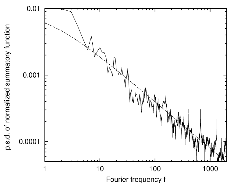
Fig. 1 shows the properly normalized period for the cycles in $\mathcal{Z}_{q}=\mathcal{Z}/q\mathcal{Z}$. Its fractal character can be appreciated by looking at the corresponding power spectral density (FFT) shown in Fig. 2. It has the form of a $1/f^{\gamma}$ noise, with $\gamma=0.70$. For a more refined link between primitive roots, cyclotomy and Ramanujan sums see also [11].

Let us remind that the algebraic equation (9) is used as a numerical trap door for public key encryption (the RSA cryptosystem) [3], p.125. While it is easy to multiply $1000$-digit numbers within a time of few milliseconds on a modern classical computer, the opposite task of factorizing is impossible in a reasonable time. This impossibility would be lifted on a quantum computer thanks to Schor’s algorithm of finding periods efficiently in $\mathcal{Z}_{q}$ (see Sect.3.3).

The quantum operator corresponding to (9) is another shift $\mu_{a}$ in the space of number states, where $a\in\mathcal{Z}_{q}$ and $(a,n)=1$. It is defined as

It is multiplicative: $\mu_{k}\mu_{l}=\mu_{kl}$ and $\mu_{k}^{*}\mu_{k}=1$, $k,l\in\mathcal{N}$. The eigenvalues and eigenvectors of the operator (10) allow to define the order $r=ord_{q}(a)$ of $a~($mod$)~q$ which is the smallest exponent such that (9) is satisfied. When the order is $r=\phi(q)$ then $a$ is a primitive root. This results from Euler theorem which states that $a^{\phi(q)}=1($mod$~q)$. If the order is the same for any $a$ such that $(a,q)=1$ it is also called a universal exponent. Thus $\phi(q)$ is a universal exponent. It is the smallest one if $a$ is a primitive root, otherwise there is a smaller one which is Carmichael lambda function introduced above. Let us summarize

The eigenvalues of operator (10) are of the form $\exp(2i\pi\frac{k}{r})$ and the corresponding eigenvectors are given as a quantum Fourier transform [12], p. 22.

We observe that (12) acts on the subspace of dimension $r$ (the least period) from the powers of $a$ in (9). One sees that the $u_{k}$’s acquire the status of phase states in the cyclic subspace of $Z_{q}$ of dimension r.

The operator $\mu_{a}$ is used in the context of quantum computation in relation to Schor’s algorithm [12]. The goal is to factor integers efficiently (in polynomial time instead of the exponential time needed on the classical computer). It is in fact related to the efficient estimation of the period $r$ taken from the eigenvalue $\exp(2i\pi\frac{k}{r})$, and to the efficient implementation of quantum Fourier transforms on the quantum computer.

The shift operator (10) which quantizes (9) plays the role of multiplication in the language of operators. The addition operator is easier to define

It encodes the individuals in the quantum Fourier transform (8). These individuals are eigenvalues of the operator $e_{p}$. One gets $e_{0}=1$, $e_{p}^{*}=e_{-p}$, $e_{l}e_{m}=e_{l+m}$. Both operators $\mu_{a}$ and $e_{p}$ form an algebra $A=(\mu_{a},e_{p})$. It was used by Bost and Connes [6],[13] to build a remarkable quantum statistical model undergoing a phase transition.

Let us now make use of the concepts of quantum statistical mechanics. Given an observable Hermitian operator $M$ and a Hamiltonian $H_{0}$ one has the evolution $\sigma_{t}(M)$ versus time $t$

and the expectation value of $M$ at inverse temperature $\beta=\frac{1}{kT}$ is the unique Gibbs state

For the more general case of an algebra of observables A, the Gibbs state is replaced by the so-called Kubo-Martin-Schwinger (or $\rm{KMS}_{\beta}$) state. One introduces a $1$-parameter group $\sigma_{t}$ of automorphisms of $A$ so that for any $t\in R$ and $x\in A$

but the equilibrium state remains unique only if some conditions regarding the evolution of the operators $x\in A$ are satisfied: the so-called $\rm{KMS}$ conditions [6]. It happens quite often that there is a unique equilibrium state above a critical temperature $T_{c}$ and a coexistence of many equilibrium states at low temperature $T<T_{c}$. There is thus a spontaneous symmetry breaking at the critical temperature $T_{c}$. A simple example is the phase diagram for a ferromagnet. At temperature larger than $T\simeq 10^{3}K$ the disorder dominates and the thermal equilibrium state is unique, while for $T<T_{c}$ the individual magnets tend to align each other, which in the three dimensional space $\mathcal{R}^{3}$ of the ferromagnet yields a set of extremal equilibrium phases parametrized by the symmetry group $SO(3)$ of rotations in $\mathcal{R}^{3}$.

In Bost and Connes approach the Hamiltonian operator is given as the logarithm of the number operator $H_{0}=\ln N$, i.e. it is a kind of “quantum Fechner law” since the “sensor” operator $H_{0}$ is the logarithm of the “physical” operator $N$, in contrast to the ordinary Hamiltonian $H_{0}=N+\frac{1}{2}$ of the harmonic oscillator. The dynamical system $(A,\sigma_{t})$ is defined by its action on the Fock states

Using the relations $e^{-\beta H_{0}}|n\rangle=e^{-\beta\ln n}|n\rangle=n^{-\beta}|n\rangle$, it follows that the partition function of the model at the inverse temperature $\beta$ is

where $\zeta(\beta)$ is the Riemann zeta function introduced at the end of Sect.2. Applying (16) to the Hamiltonian $H_{0}$ in (17) one gets

One observes that under the action of $\sigma_{t}$ the additive phase operator (13) is invariant, while the multiplicative shift operator (10) oscillates in time at angular frequency $\ln a$. It is found in [6],[13] that the pole $\beta=1$ of the Riemann zeta function separates two dynamical regimes.

In the high temperature regime $0<\beta\leq 1$ there is a unique $\rm{KMS}_{\beta}$ state of the dynamical system $(A,\sigma_{t})$. The expectation value $\psi_{\beta}(\frac{p}{q})$ for the irreducible fractions $\frac{p}{q}$, $(p,q)=1$ is

and the $k_{b}$ are the exponents in the unique prime decomposition of the denominator $q$

In the low temperature regime $\beta>1$ things become more involved. The $\rm{KMS}_{\beta}$ state is no longer unique, as it is in the case of the low temperature ferromagnet. The symmetry group $G$ of the dynamical system ($A,\sigma_{t}$) is a subgroup of the automorphisms of $A$ which commutes with $\sigma_{t}$

where $\circ$ means the composition law in $G$. When the temperature is high the system is disordered enough that there is no interaction between its constituents and the equilibrium state of the system does not see the action of the symmetry group $G$, which explains why the thermal state is unique. At lower temperature $T<T_{c}$ the constituents of the system may interact. The symmetry group $G$ then permutes a family of extremal $\rm{KMS}_{\beta}$ states generating the possible states of the system after phase transition. The symmetry group for the algebra $A=(\mu_{a},e_{p})$ and the “quantum Fechner Hamiltonian” $H_{0}$ in (17) is the Galois group $G=Gal(\mathcal{Q}^{\rm{cycl}}/\mathcal{Q})$ of the cyclotomic extension $\mathcal{Q}^{\rm{cycl}}$ of $\mathcal{Q}$. The field $\mathcal{Q}^{\rm{cycl}}$ is the one generated on $\mathcal{Q}$ by all the roots of unity. The Galois group $G$ is the automorphism group of $\mathcal{Q}^{\rm{cycl}}$ which preserves the sub-field $\mathcal{Q}$. It is isomorphic to $\mathcal{Z}_{q}=(\mathcal{Z}/q\mathcal{Z})^{*}$ which is the group of integers modulo $q$ with the zero element removed.

One immediately sees that the action of the Galois group $G$ commutes with the $1$-parameter group defined in (19). Hence $G$ permutes the extremal $\rm{KMS}_{\beta}$ states of $(A,\sigma_{t})$. To describe these thermal states for $\beta>1$ one starts from the action of operators $\mu_{a}$ and $e_{p}$ on Fock states as given in (10) and (13), and one allows the permutation by the symmetry group $G$. For each $w\in G$, one has a representation $\pi_{w}$ of the algebra $A$ so that

and it is shown in [6] that the state

is a $\rm{KMS}_{\beta}$ state for $(A,\sigma_{t})$. The action of $G$ on $A$ induces an action on these thermal states which permutes them. For $\beta>1$ the expectation value acting on the phase operator $e_{p}$ may be written as $\rm{KMS}(e_{p})=q^{-\beta}\prod_{\stackrel{{\scriptstyle p~\rm{divides}~q}}{{p~\rm{prime}}}}\frac{1-p^{\beta-1}}{1-p^{-1}}$. But it can be also found that formula (20) is valid in the whole range of temperatures $0\leq\beta\leq\infty$.

Plotting the thermal state (Fig. 3) one observes the following asymptotes. In the high temperature limit $\beta$=0 the thermal state tends to $1$; in the low temperature range $\beta\gg 1$ the thermal state is well approximated by the function $\mu(q)/\phi(q)$, where the Möbius function $\mu(q)$ is $0$ if the prime decomposition of $q$ contains a square, $1$ if $q=1$ and $(-1)^{k}$ if $q$ is the product of $k$ distinct primes. Close to the critical temperature at $\beta=1$ the fluctuations are squeezed and the thermal state is quite close to $\epsilon\Lambda(q)/q$, when $\epsilon=1-\beta\rightarrow 0$, where $\Lambda(q)$ is the Mangoldt function defined in (3). It is an unexpected surprise that phase fluctuations at the critical region of the quantum perception model resembles the ones of the classical phenomenological model of time measurements.

It is shown in our earlier papers [2], in eq. (38) that the normalized Möbius function $\mu(q)/\phi(q)$ is the dual to the Mangoldt function $\Lambda(n)$ when one projects on to the basis of Ramanujan sums. Ramanujan sums $c_{q}(n)$, which are defined as the sums of $n^{\rm{th}}$ powers of primitive roots of unity, generalize the cosine function, being quasi-periodic in $n$ and aperiodic in $q$. The thermal states in the transition region can thus be considered as an unfolding through the dimensions $q$ of the unique high temperature thermal state. This also suggests to consider the inverse temperature $\beta$ and the dimension $q$ of the Hilbert space as complementary to each other in the Heisenberg sense.

We tried to make clear that time perception is the quantum counterpart to time measurements. The quantum algebra of shift and clock operators together with the “quantum Fechner law” lead to well defined thermal perception states, that should play some role in memory encoding and conscious activity. There seems to be a growing consensus that the mental activity in brain doesn’t relate to classical synchronization rules in neurons, but to some other non local mechanism at a smaller scale, possibly at the mesoscopic scale of microtubules within neurons [14],[15],[16].

Quantum field theory of many body systems and the mechanism of spontaneous breakdown of symmetry was already proposed to accommodate some features of the conscious brain function. Memory recording was represented by the ordering induced in the ground state by the condensation of modes after symmetry breaking of the rotational symmetry of the electrical dipoles of the water molecules. The recall mechanism was described by the excitation of these collective modes from the ground state under the action of an external input similar to the one which was previously produced by memory encoding. In a dissipative extension of the model two modes squeezed coherent states of the radiation field were found to play a role in extending considerably the memory capacity [17].

The set of collective modes in the ground sate of Vitiello’s model is replaced in our model by the set of thermal phase states (the extremal $\rm{KMS}_{\beta}$ states). Transitions among the vacua are replaced by transitions among the $\rm{KMS}_{\beta}$ states under the action of the cyclotomic group. Vitiello’s model can be seen as an attempt to include the environment in the quantum model of brain, thus the idea of two entangled modes, one in the brain, the other one in the environment. Our approach seems more general being able to describe the environment thanks to a continuous temperature parameter $\beta$, and putting on the scene more general squeezed thermal states at the transition temperature. The discrete parameter $q$ is the dimension of the Hilbert space of Fock states. It plays the role of a bandwidth in conscious and unconscious activity. A very wide bandwidth $q\rightarrow\infty$ would mean meditation, a small bandwidth would be associated to precise memory encoding, jumps between dimensions, with tiny energy needed, thanks to the ridges of the $\rm{KMS}$ versus $q$ and $\beta$ diagram (see. Fig. 3). Another closely related view of time perception based on cyclic properties of Galois Fields $GF(b^{k})$ has been proposed [18]. This pencil model sheds new light on profoundly distorted perceptions of time characterizing a number of mental psychoses, drug-induced states, as well as many other “altered” states of consciousness. The high temperature thermal state could be associated to the ordinary sense of time, and the low temperature thermal states to altered states of time perception.

References

- [1] B. Flanagan. Are perception fields quantum fields? NeuroQuantology 2003; 3:334-364.
- [2] M. Planat. Invitation to the “spooky” quantum phase-locking effect and its link to fluctuations. Preprint 2003; arXiv:quant-ph/0310082.
- [3] M. R. Schroeder. Number Theory in Science and Communication. Berlin: Springer 1999; 16-24.
- [4] D. L. Gilden. Cognitive emissions of noise. Psychological Review 2001; 108:33-56.
- [5] H. Poincaré. Mathematical magnitude and experiment. Chapter 2 in Science and Hypothesis. London: Walter Scott Publishing 1905; 17-34.
- [6] J. B. Bost and A. Connes. Hecke algebra, type III factors and phase transitions with spontaneous symmetry breaking in number theory. Selecta Mathematica 1995; 1: 411-457.
- [7] R. Lynch. The quantum phase: a critical review. Physics Reports 1995; 256: 367-436.
- [8] A. Vourdas. Phase states: An analytic approach in the unit disk. Physica Scripta 1993; T48: 84-86.
- [9] A. Perelomov. Generalized Coherent States and Their Applications. Berlin: Springer Verlag 1986.
- [10] V. Bouchiat, D. Vion, P. Joyez, D. Estéve and M. H. Devoret. Quantum coherence with a single Cooper pair. Physica Scripta 1998; 1: 165-170.
- [11] P. Moree P and H. Hommerson H. Value distribution of Ramanujan sums and of cyclotomic polynomial coefficients. Preprint 2003; math.NT/0307352
- [12] A. Ekert, P. Hayden and H. Inamori. Basic concepts in quantum computation. in Coherent Atomic Matter Waves. Les Houches Summer School. Berlin: Springer 2001. Preprint 2000; quant-ph/0011013.
- [13] P. B. Cohen. Dedekind zeta functions and quantum statistical mechanics. Contemporary mathematics 1999; 241: 121-128.
- [14] M. Jibu, S. Hagan, S. R. Hameroff, K. H. Pribam and K. Yasue. Quantum optical coherence in cytoskeletal microtubules: implications for brain function. Biosystems 1994; 32: 195-209.
- [15] D. V. Nanopoulos. Theory of brain function, quantum mechanics and superstrings. CERN-TH 1995; 95-128. Preprint 1995; hep-ph/9505374.
- [16] H. Rosu. Essay on mesoscopic and quantum brain. Metaphysical Review 1997; 3:1-12. Preprint 1997; gr-qc/9409007.
- [17] G. Vitiello. Dissipation and memory capacity in the quantum brain model. Int. J. Mod. Phys. 1995; 9: 973-989.
- [18] M. Saniga, Pencils of conics: a means towards a deeper understanding of the arrow of time? Chaos, Solitons and Fractals 1998; 9: 1071-1086. Also: Temporal dimension over Galois fields of characteristic two. Chaos, Solitons and Fractals 1998; 9: 1095-1104.