SUNYB/04-03, IP/BBSR/04-05, August 11, 2026
Periodic Potentials and Supersymmetry
Avinash Kharea,11 1 khare@iopb.res.in and Uday Sukhatmeb,22 2 sukhatme@buffalo.edu
a)
Institute of Physics, Sachivalaya Marg, Bhubaneswar 751005, Orissa, India
b)
Department of Physics, State University of New York at Buffalo,
Buffalo, NY 14260, U.S.A.
I. INTRODUCTION
One dimensional potential wells have bound states. They are solutions of the Schrödinger equation which satisfy appropriate boundary conditions. When two identical potential wells are very far apart, then each potential has the same energy levels, and each eigenstate is doubly degenerate. As the wells are brought closer together, there is communication between them, and each level is split into two. Similarly, if one has an array of many identical wells making a periodic potential, then one gets energy bands, which play, for example, a crucial role in determining the electronic properties of crystalline solids. To illustrate this band structure qualitatively, condensed matter physics texts usually treat the problem of a one dimensional periodic array of delta functions, called the Kronig Penney model. Here, one gets a transcendental equation for computing band edges. Another well-studied class of periodic potentials are the Lamé potentials [1, 2, 3]
| (1) |
where is a Jacobi elliptic function [4] of real elliptic modulus parameter m (). If is any positive integer, it is well known that these potentials have only band gaps and hence band edges which are analytically known (in principle). However, this is an exceptional example. The bottom line is that even in one dimension, there are very few solvable periodic potentials, and it would be desirable to have more, especially some with a richer spatial structure.
We shall describe how to obtain new solvable periodic potentials via several different approaches. One way, for example is to expand our knowledge of Lamé potentials to the wider class of associated Lamé (AL) potentials [5, 6]
| (2) |
where are constants and without any loss of generality we consider . A second way, for example is to exploit the fact that Jacobi elliptic functions are doubly periodic functions and consider PT-invariant complex periodic potentials [7] obtained from the Lamé and the AL potentials by considering the anti-isospectral transformation (where is any nonzero real number) [8]. A third way is to consider a linear superposition of several Lamé (AL) potentials which in view of the Landen transformations [9, 10] and cyclic identities [11] for Jacobi elliptic functions can be shown to be essentially equivalent to Lamé (AL) potentials with modified parameters. Finally, we can further expand all these classes of solvable potentials by using the techniques of supersymmetric quantum mechanics to generate supersymmetric partner potentials [12].
The outline of this paper is as follows. In Sec. II we review some general properties of periodic potentials as well as the relevant formalism of supersymmetric quantum mechanics. In Sec. III we discuss the band edge energies and eigenfunctions for several Lamé and AL potentials. In particular, for Lamé potentials (1) we derive a remarkable hitherto un-noticed relation connecting band edge energy eigenstates corresponding to modulus parameters and . We also describe how the Lamé potential results can be vastly expanded to get solutions for the AL potentials (2). In particular, we show that for any integral with , there are bound bands followed by a continuum band, out of which the top bound bands are unusual in the sense that both band edges are of period ()) when the integer is even(odd), where is the complete elliptic integral of the first kind. In Sec. IV we obtain the supersymmetric partners of both the Lamé and the AL potentials, thereby expanding the list of solvable periodic potentials. In Sec. V we show that using Landen transformations [10] and cyclic identities obtained by us recently [11], exact band edge eigenvalues and eigenfunctions can also be obtained in the case of linear superposition of Lamé and AL potentials. In Sec. VI we show that a class of PT-invariant complex periodic potentials obtained from the Lamé and AL potentials by the anti-isospectral transformation , ( being any nonzero real number) are also exactly solvable problems with real band spectra. Finally, in Sec. VII we discuss the double sine-Gordon equation and show that in some special cases it has unusual band spectra, in that the majority of bound bands have both of their band edges of the same period.
II. GENERAL PROPERTIES
(a) Periodic Potentials: For a real potential with period , one is seeking solutions of the Schrödinger equation subject to the Bloch condition
| (3) |
where denotes the crystal momentum. The spectrum shows energy bands whose edges correspond to , that is the wave functions at the band edges satisfy . For periodic potentials, the band edge energies and wave functions are often called eigenvalues and eigenfunctions, and we will also use this terminology.
A general property of eigenstates for a real potential with period is the oscillation theorem. It states that band edge wave functions, when arranged in order of increasing energy , have periods [1]. The corresponding number of wave function nodes in the interval are and the energy band gaps are given by . The oscillation theorem is very useful in identifying if all band edge eigenstates have been properly determined or if some have been missed.
(b) Supersymmetric Quantum Mechanics: The supersymmetric partner potentials are defined in terms of the superpotential by [12]
| (4) |
where (by convention) the superpotential is related to the ground state eigenfunction of by
| (5) |
The corresponding Hamiltonians can be factorized as
| (6) |
where
| (7) |
so that the spectra of are nonnegative. It is also clear that on the full line, both cannot have zero energy modes, since the two functions given by
| (8) |
cannot be simultaneously normalized.
On the other hand, when the superpotential has period [], and the eigenfunctions of both must satisfy the Bloch condition (3), it is easily shown that in the periodic case, irrespective of whether supersymmetry is broken or unbroken, the spectra of are strictly identical [13, 14]. Further, one has unbroken supersymmetry provided
| (9) |
and in this case the partner Hamiltonians have identical spectra including zero modes and both belong to the Hilbert space. As a result, unlike on the full line, for periodic potentials, whenever the condition (9) is satisfied, supersymmetry is unbroken and yet the Witten index (which counts the difference between the number of zero modes of ) is always zero.
The condition (9) is trivially satisfied when is an odd function of and throughout this paper we shall only consider superpotentials which are odd function of . Further, using the known eigenfunctions of , one can immediately write down the corresponding eigenfunctions of . In particular, from eq. (8) it follows that the ground state of is given by [12]
| (10) |
while the un-normalized excited states are obtained from by using the relation
| (11) |
Thus by starting from an exactly solvable periodic potential , one gets a new isospectral periodic potential .
A few years ago, the concept of self-isospectral periodic potentials has been defined and developed in detail [13]. A one dimensional potential of period is said to be self-isospectral if its supersymmetric partner potential is just the original potential upto a discrete transformation - a translation by any constant amount, a reflection, or both. A common example is translation by half a period, in which case the condition for self-isospectrality is In this sense, any self-isospectral potential is rather uninteresting, since the application of supersymmetry just yields a discrete transformation and basically nothing new.
III. LAMÉ AND ASSOCIATED LAMÉ POTENTIALS
(a) Lamé Potentials: The Lamé potentials as given by eq. (1) have a period . Their name comes from the fact that the corresponding Schrödinger equation (with )
| (12) |
is called Lamé equation [1, 2]. It is well known that for any integer value , the corresponding Lamé potential has bound bands followed by a continuum band [1, 2] and the band edge energy eigenstates are analytically known in principle. We now obtain remarkable new relations (valid for any integer ) relating the band edge energy eigenvalues and eigenfunctions at two values and of the modulus parameter.
We start from the Schrödinger equation (12). On using the relation [4]
| (13) |
and defining a new variable , the Schrödinger eq. (12) takes the form
| (14) |
On comparing eqs. (12) and (14) we then have the desired relations relating the eigenstates when the modulus parameter is and :
| (15) |
Thus, for any integer , at , one has remarkable relations
| (16) |
On using
| (17) |
one can immediately and explicitly verify the relations (15) and (S0.Ex1) for .
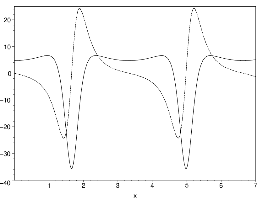
For the = 2 case, the Lamé potential has 2 bound bands and a continuum band. The energies and wave functions of the five band edges are well known [1, 2]. The lowest energy band ranges from to , the second energy band ranges from to and the continuum starts at energy , where . For subsequent application of the supersymmetric quantum mechanics formalism, it is convenient to have a potential whose ground state energy is zero. This is easily accomplished via a re-defined potential with the ground state energy subtracted out. For the problem under consideration, one has . This potential is plotted in Fig. 1. The eigenstates of all the band edges are given in Table 1. Note that in the interval corresponding to the period of the Lamé potential, the number of nodes increases with energy, in agreement with the oscillation theorem. From Table 1, it is easy to check that, as expected, the relations (15) and (S0.Ex1) are indeed true.
We might add here that in case is not an integer, then for Lamé potentials one has an infinite number of bands and band gaps for which (to the best of our knowledge) no analytic results are available. However, when is half-integral, then mid-band levels are in principle analytically known and each of them is doubly degenerate [1, 2].
(b) Associated Lamé Potentials: We now expand our discussion to the band edges and wave functions of a much richer class of periodic potentials given by eq. (2) called associated Lamé (AL) potentials, since the corresponding Schrödinger equation is called the associated Lamé equation [1]. More precisely, we often refer to the AL potential of eq. (2) as the potential where and and note that potentials are just the ordinary Lamé potentials. The AL potentials (2) can also be re-written in the alternative form [4, 5]. Clearly, the potentials and have the same energy spectra with wave functions shifted by . Therefore, it is sufficient to restrict our attention to , i.e. .
In general, for any values of and , the AL potentials have a period , but for the special case the period is From a physical viewpoint, if one thinks of a Lamé potential as due to a one-dimensional regular array of atoms with spacing and “strength” , then the AL potential results from two alternating types of atoms spaced by with “strengths” and respectively. If the two types of atoms are identical [which makes ], one expects a potential of period .
Extrema (defined for this discussion as either local or global maxima and minima) of AL potentials are easily found by setting Extrema occur when , or . Also, for fixed values of and , there are additional extrema if lies in the critical range
The AL potentials for and several values of are plotted in Fig. 2. In the critical range of values one expects additional extrema, and these are clearly seen.
(c) Parabolas of Solvability: The AL equation is
| (18) |
On substituting it is easily shown that , satisfies the Hermite elliptic equation [1]. On further substituting one obtains Ince’s equation
| (19) |
where
| (20) |
which is a well known quasi exactly solvable equation [1]. In particular if ( ) then one obtains solutions, which are given in Table 2. In particular, for any given choice of Table 2 lists the eigenstates of the AL equation for various values of .
For , there is just one eigenstate with energy and wave function . Since the wave function has period and is nodeless, this is clearly the ground state wave function of the potential for any real choice of the parameter . The equations and are the parametric forms of the equation of the parabola , which is plotted in Fig. 3 and labeled . For any point on the parabola, one knows the ground state wave function and energy . The parabola includes the points (2,0) and (6,2).
For , we see from Table 2 that two eigenstates with energies and are known. Since they have period and just one node in the interval , they must correspond to the first and second band edge energies and of the potential. Eliminating from the equations and gives the “parabola of solvability” , which is plotted in Fig. 3 and labeled . This parabola includes the points (2,0) and (6,0) which correspond to Lamé potentials. Similarly, the parabolas of solvability corresponding to in Table 2 are plotted. Note that eigenstates are known for any point on the parabola of solvability .
All Lamé as well as AL potentials for which are unequal integers, have two parabolas of solvability passing through. This provides a good understanding of why these are completely solvable problems. For instance, the potential is at the intersection of parabolas P1 (1 known state) and P2 (2 known states), thus giving the 3 known band edges. Similarly, the AL potential. lies on parabola P1 (1 known nodeless state of period ) and parabola P4 (4 known states of period , two with 1 node and two with 3 nodes). Since we know from the oscillation theorem that 2 states of period are missing, so it would appear that this is an example of a quasi exactly solvable potential. However, using a well known theorem about Ince’s equation [1] we discuss below that the two “missing” states are degenerate and have no band gap between them. Hence, AL potentials are also exactly solvable periodic problems with a finite number of band gaps when both and are unequal positive integers.
Other fully solvable examples correspond to AL potentials with integer. For example, the potential has period . It lies on parabola P3 (3 known states) and the band edge periods are . We shall discuss these examples in some detail in Sec. V where we show that in view of the Landen transformation formulas for Jacobi elliptic functions, these problems are essentially related to Lamé potentials with integer and hence exactly solvable.
(d) Exact Results: Several exact results are known in the literature about the Ince’s equation (19). In particular, it is well known that the system satisfying Ince’s eq. (19) has at most band gaps of period ] in case the polynomial defined by
| (21) |
where are as given by eq. (S0.Ex4) has either non-negative integral roots, the highest of which is , or negative integral roots, the lowest of which is . The fact that the Lamé potentials (1) have only band gaps when is any positive integer is easily understood from here. We now show [6] that on applying this theorem, one can draw the following conclusions about the associated Lamé potentials:
- 1.
unequal positive integers: In this case one can show that for , there are only bound bands followed by a continuum band out of which the lowest bands are normal bands with one band edge wave function of period and the other with period , while the top bound bands are unusual in that both of their band edges are of period in case is an even [odd] integer. Further, all the band edge eigenvalues and eigenfunctions are in principle known analytically. As an illustration, in Table 3 we have given all five band edge energy eigenstates of the potential.
- 2.
Both being half-integral: In this case there are infinite number of bands and band gaps. However, but for the lowest bands, the rest are unusual in that both of their band edges are of period in case is an even [odd] integer. Further, in this case band edge energy eigenstates of period are analytically known in principle, in case is an odd [even] integer. Besides, one also analytically knows the energy eigenvalues and eigenfunctions of mid-band states of period each of which is doubly degenerate in case is an odd [even] integer [6].
- 3.
Either or integral: When neither nor is integral or half-integral but either their sum or difference is an integer, then one again has infinite number of bands and band gaps. Further, one can show that if either or , then there are at most band gaps of period and one analytically knows the energy eigenvalues and eigenfunctions of band edges of period . On the other hand, if or , then there are at most band gaps of period and one has analytical expressions for band edges of period .
Finally, just as mid-band states, with each being doubly degenerate, are analytically known in case parameter of the Lamé potential (1) is half integral, one can show that a similar number of doubly degenerate mid-band states are also known for every integral value of in the case of AL potentials (2) with half-integral [6].
IV. SUPERSYMMETRIC PARTNER POTENTIALS:
(a) Lamé potentials: Let us first apply the supersymmetric quantum mechanics formalism as explained in Sec. II to the Lamé potentials (1) when is positive integer. Since analytic solutions are known for integer values of [2], the supersymmetric partner potentials can be readily computed using eqs. (4) and (5). We first discuss the results for small integer values of , and then present some eigenstate results for arbitrary integer values of .
In order to use the supersymmetry formalism, we must shift the Lamé potential by a constant to ensure that the ground state i.e. (the lower edge of the lowest band) has energy . For , one has and the superpotential is . The partner turns out to be just , so that this is an example of self-isospectrality. For , the potential is
| (22) |
with a unnormalized ground state wave function [2]. The corresponding superpotential is
| (23) |
and hence the partner potential for the potential given in eq. (22) is
| (24) |
Although supersymmetry guarantees that the potentials are isospectral, in this example they are not self-isospectral. Therefore, as given by eq. (24) is a new periodic potential which is strictly isospectral to the potential (22) and hence it also has 2 bound bands and a continuum band. In Fig. 1 we have plotted the potentials corresponding to for . Using eqs. (10) and (11) and the known eigenstates of , we can immediately compute all the band-edge Bloch wave functions for . In Table 1 we have given the energy eigenvalues and wave functions for the isospectral partner potentials . In summary, for integral , Lamé potentials with are not self isospectral. They have distinct supersymmetric partner potentials even though both potentials have the same band edge eigenvalues.
(b) Associated Lamé potentials: It is easily checked from Table 2 that the solution corresponding to as well as one of the solutions are nodeless and correspond to the ground state. Hence, for these cases, one can obtain the superpotential and hence the partner potential . For example, consider the case of . In this case is given by so that the corresponding partner potentials are
These partner potentials are self-isospectral and so supersymmetry yields nothing new. As an illustration, the potential (6,2) as discussed in Table 3 is a self-isospectral potential and supersymmetry yields nothing new.
Let us now consider the partner potential computed from the ground state for the case. Here , where . The corresponding superpotential turns out to be
| (25) |
Hence the corresponding partner potentials are
| (26) |
These potentials are not self-isospectral. Thus one has discovered a whole new class of periodic potentials for which three states are analytically known no matter what is. In particular, the energy eigenfunctions of these three states are easily obtained by taking the corresponding energy eigenstates of as given in Table 2 and using eqs. (10) and (11).
We might add here that applying second order Darboux transformations to the Lamé potentials, Fernández et al [15] have obtained an interesting nonlocal effect, by which the transformed potential becomes an exact or approximately displaced copy of the original one.
V. SUPERPOSITION OF LAMÉ AND ASSOCIATED LAMÉ POTENTIALS
Using the recently discovered cyclic identities [11] and Landen transformation formulas [9, 10] for Jacobi elliptic functions, we shall now further expand the list of analytically solvable periodic potential problems. In particular, we obtain the exact band edge eigenstates for potentials obtained via a certain specific type of linear superposition of Lamé as well as AL potentials.
Superposition of Lamé potentials: Consider the following linear superposition of Lamé potentials with translated arguments:
| (27) |
where . Note that for the special case of , this corresponds to the AL potential with . On expressing in terms of , the corresponding Schrödinger equation is given by
| (28) |
On making use of the Landen transformation formula [9, 10]
| (29) |
where
| (30) |
and
| (31) |
one can rewrite the Schrödinger eq. (28) in the form
| (32) |
Here . Using recently discovered cyclic identities, can be shown to be [11]
| (33) |
where , while is the Jacobi zeta function [4]. On making the transformation , the Schrödinger eq. (32) can be rewritten as a Lamé equation but for the modulus parameter and with energy :
| (34) |
Here the true energy eigenvalues of the superposed potentials (27) are related to the eigenvalues of the Lamé potentials by
| (35) |
where and are as given by eqs. (30) and (S0.Ex6) respectively while and are related by eq. (31). Similarly, the true eigenfunctions of the superposed potentials (27) are related to those of eq. (34) by
| (36) |
As an illustration, for (i.e. AL case), it is well known [9, 10] that
| (37) |
and hence the energy eigenvalues of the AL potentials (27) (with ) are given in terms of those of Lamé potential (1) (but with the modulus parameter ) by
| (38) |
For we can immediately verify that the energy eigenvalues and eigenfunctions of the (2,2) and (6,6) potentials as calculated from here are identical (as they should be) to those calculated by us by an entirely different method where no use of either Landen transformations or the cyclic identities was made [5].
In fact we can relate the energy eigenstates of the AL potentials at different modulus parameters by using the relationship (15) between the corresponding Lamé energy eigenstates. For this purpose, it is best to reexpress the relation (38) entirely in terms of by noting that on using eq. (37) we have
| (39) |
Using eqs. (37) to (39) in eq. (15) we find that the AL eigenvalues are related by (where for simplicity we have replaced everywhere by )
| (40) |
where
| (41) |
For we immediately verify that these relations are indeed true. Further, the corresponding eigenfunctions are related by
| (42) |
where .
Similarly, for , it is well known that
| (43) |
and hence the energy eigenvalues of (27) (with ) are given in terms of those of Lamé’s with parameter by
| (44) |
Thus by using Landen transformations and recently discovered cyclic identities one has discovered new solvable periodic potentials. On following the last section, it is easy to see that for any integer , corresponding to every superposed potential, supersymmetry will give us another new exactly solvable periodic potential.
Superposition of Associated Lamé potentials: Consider the the following superposition of AL potentials
| (45) |
where . Now proceeding exactly as above and using the Landen transformation (29) and the cyclic identity (S0.Ex6), one can show that the energy eigenvalues and eigenfunctions of the superposed AL potentials (45) are related to those of AL potential (2) (but with modulus parameter ) by
| (46) |
| (47) |
where and are given by eqs. (30), (31) and (34) respectively. Thus we have further enlarged the list of new exactly solvable periodic problems. Needless to say that using supersymmetry, one can further enlarge this list by obtaining partner potentials of the superposed potentials which will have the same band spectra.
As an illustration, for , the energy eigenvalues of the superposed potentials (45) are given below in terms of the corresponding AL potentials (with modulus parameter changed to ):
| (48) |
| (49) |
VI. PT INVARIANT POTENTIALS WITH REAL BAND SPECTRA
We shall now show that the complex PT-invariant periodic potentials obtained by applying the anti-isospectral transformation [16] (where is a nonzero real number) to the Lamé and AL potentials with a finite number of band gaps are also exactly solvable and have a finite number of band gaps. We give explicit expressions for the band edges of some of these potentials [8]. For the special case of the potential , we analytically obtain the corresponding dispersion relation.
Let us begin with the simple observation that if is a solution of the Schrödinger equation for the real potential with energy , then is a solution of the Schrödinger equation for the complex potential with energy . The new potential , generated by the anti-isospectral transformation , is clearly PT-symmetric and will be denoted by .
It is important to understand that the key point in obtaining these results is that unlike trigonometric and most other periodic functions, the Jacobi elliptic functions are doubly periodic functions. This allows both and to be simultenously periodic, even though the periods are different. Note that the arbitrary nonzero constant in the transformation helps us to avoid the singularities of Jacobi elliptic functions.
Let us first apply our approach to the Lamé potentials (1). On applying the anti-isospectral transformation [16], where is any non-zero real number, it is easily shown that the band-edge eigenvalues and eigenfunctions of the PT-invariant potentials
| (50) |
are related to those of the Lamé potentials (1) by [8]
| (51) |
It may be noted here that the PT-invariant complex potential (50) is a periodic potential with period . Thus we have shown that the PT-invariant periodic potential (50) too has precisely band gaps and hence band edges at energies given by relation (51). Special mention may be made of the remarkable fact that for any integer , all bands and band gaps exchange their role as one goes from a Lamé potential to its PT-transformed version.
For any band structure problem, one important quantity is the discriminant [1] which gives information about the number of band gaps as well as their widths. The question is if we can relate with the discriminant for the corresponding Lamé potential. We now show that using eqs. (15) and (51) this is indeed possible. In particular, on using these two equations we deduce that
| (52) |
and hence the corresponding discriminants are related by [8]
| (53) |
As an illustration, in Fig. 4 we plot the real and imaginary parts of the PT-invariant complex potential . Using the well known results for the Lamé potential with (see Table 2) and eq. (51), the ground state (lowest band edge) eigenvalue and eigenfunction is easily shown to be
| (54) |
where . In Table 4 we have given all the five band edge eigenvalues and eigenfunctions of this PT-invariant potential, where we have subtracted off the ground state energy from the potential so that the lowest band edge by construction is at zero energy. Observe from the table that the band edges are both periodic as well as anti-periodic with periods of and respectively thereby showing that contrary to the suggestion of Bender et al. [17], the absence of anti-periodic band edges is not a general property of PT-invariant periodic potentials.
Additional analytically solvable finite band gap potentials can be obtained from here by using supersymmetry. In particular, consider the potential . Its ground state eigenfunction is given in eq. (54), and we find that the corresponding superpotential is
| (55) |
Thus the supersymmetric partner potential is
| (56) |
and it has the same energy spectrum as [see Table 4]. In this way, one has discovered yet another PT-invariant complex potential with a finite number of band gaps. The corresponding band edge energy eigenfunctions are immediately obtained from those of by using supersymmetry transformations given in Sec. II.
Yet another complex PT-invariant potential having the same band edge eigenvalues as above is obtained by starting from the partner potential of the Lamé potential [eqs. (24) and (22)] and then obtaining the corresponding PT-invariant potential by the anti-isospectral transformation . Thus one has found three distinct complex PT-invariant periodic potentials having the same band spectra. One can show that this is true for any integral . On the other hand, for one can show [8] that the three potentials are not distinct but are self-isospectral (i.e. differ from each other by a translation by a constant) [13, 15].
For the special case of the Lamé potential, the dispersion relation is analytically known [3]. We now show [8] that it is possible to derive the dispersion relation for the PT-invariant potential (50) with . To that end we start from the Schrödinger equation:
| (57) |
where we have subtracted the ground state energy from the potential so that the new potential has zero ground state energy. On substituting , eq. (57) takes the form
| (58) |
Now it is well known that two independent solutions of this equation are given by [3]
| (59) |
where are Jacobi eta, theta and zeta functions while is related to of eq. (57) by
| (60) |
On using the fact that while is periodic function with period , is only quasi-periodic [3], i.e.
| (61) |
and using the Bloch condition, it is easily shown that for the PT-invariant complex potential (1) with , the dispersion relation is given by
| (62) |
where is given by eq. (60).
We now turn to the associated Lamé potentials given by eq. (2) where without any loss of generality we consider with both being positive integers. On using the anti-isospectral transformation, it is easy to see that the band edges of the potential (2) and its PT-transformed one as given by
| (63) |
are again related by the relation (51).
For the special case , using relations (39),(40) and (51) we obtain an interesting relation betwen the eigenvalues of the AL potential and the corresponding complex PT-invariant potential given by
| (64) |
where are as defined by eq. (41). Hence we can immediately relate the discriminant for the AL potential and the corresponding complex PT-invariant potential, i.e. we have
| (65) |
VII. UNUSUAL BAND STRUCTURE FOR THE DOUBLE SINE-GORDON EQUATION
Finally, we would like to consider the band spectra of the double sine-Gordon equation characterized by the periodic potential
| (66) |
where are real, and without loss of generality is taken to be nonnegative. This equation arises in several areas of condensed matter physics. It is well known that this system has an infinite number of bands and band gaps. Further, it is also well known that if is an integer then band edges of period () are analytically known depending on whether is an odd(even) integer [18, 19]. However, what is not so well known [1] is that in case is an integer, then the potential has unusual band spectra.
We start from the Schrödinger equation for the potential (66). On using the ansatz
| (67) |
in the Schrödinger equation, it is easily shown that satisfies Ince’s eq. (19)
| (68) |
As discussed before, this is a quasi-exactly solvable equation, i.e. band edges of period ) are analytically known when is an odd (even) integer [18, 19]. We can now compute the polynomials and defined in eq. (21), and from them we conclude that if is an odd (even) integer then there are at most band gaps of period ).
It is worth pointing out here that similar conclusions can also be drawn about the complex PT-invariant periodic potential
| (69) |
Note that this potential is invariant under the parity transformation followed by . As has been shown in ref. [19], when is an even integer then PT symmetry is spontaneously broken and there are no quasi-exactly solvable states of period since in this case all the eigenvalues are now complex conjugate pairs. However, if is an odd integer then there are quasi-exactly solvable states of period and in this case PT symmetry is not spontaneously broken. On completing the above analysis, it follows that if is an odd integer then there are at most band gaps of period . Thus in this case the band spectrum is rather unusual in that the majority of the infinite number of band edges are anti-periodic and have period , thereby again showing that the absence of anti-periodic band edges is not a characteristic feature of PT-invariant potentials.
Acknowledgements: It is a pleasure to thank the U.S. Department of Energy for partial support of this research.
References
- [1] W. Magnus and S. Winkler, Hill’s Equation (Wiley, New York, 1966).
- [2] F. M. Arscott, Periodic Differential Equations (Pergamon, Oxford, 1981).
- [3] E. T. Whittaker and G. N. Watson, A Course of Modern Analysis (Cambridge Univ. Press, Cambridge, 1980).
- [4] For the properties of Jacobi elliptic functions, see, for example, I. S. Gradshteyn and I. M. Ryzhik, Table of Integrals, Series and Products ( Academic Press, 20000); M. Abramowitz and I. Stegun, Handbook of Mathematical Functions (Dover, 1964). The modulus parameter is often called in the mathematics literature. The related complementary quantity is often called .
- [5] A. Khare and U. Sukhatme, Jour. Math. Phys. 40, 5473 (1999).
- [6] A. Khare and U. Sukhatme, Jour. Math. Phys. 42, 5652 (2001).
- [7] C.M. Bender and S. Boettcher, Phys. Rev. Lett. 80, 5243 (1998), For a recent review of this field, see C.M. Bender, D.C. Brody and H.F. Jones, Amer. J. Phys. 71, 1095 (2003) and references therein.
- [8] A. Khare and U. Sukhatme, math-ph/0402006.
- [9] See for example, D.F. Lawden, Elliptic Functions and Applications, Applied Math. Sc. Vol. 80 (Springer, 1989); A. Cayley, An Elementary Treatise on Elliptic Functions (G. Bell, 1895).
- [10] A. Khare and U. Sukhatme, math-ph/0208004.
- [11] A. Khare and U. Sukhatme, Jour. Math. Phys. 43, 5652 (2001); A. Khare, A. Lakshminarayan and U. Sukhatme, ibid 44, 1841 (2003); math-ph/0306028.
- [12] See, for example, F. Cooper, A. Khare and U. P. Sukhatme, Phys. Rep. 251, 267 (1995).
- [13] G. Dunne and J. Feinberg, Phys. Rev. D57, 1271 (1998).
- [14] Y. Brihaye and M. Godart, J. Math. Phys. 34, 5283 (1993); Y. Brihaye and S. Braibant, J. Math. Phys. 34, 2107 (1993); H. Braden and A. Macfarlane, J. Phys. A18, 3151 (1995); G. Dunne and J. Mannix, Phys. Lett. B428, 115 (1998).
- [15] D.J. Fernández, B. Mielnik, O. Rosas-Ortiz and B.F. Samsonov, Phys. Lett. A294, 168 (2002); J. Phys. A35, 4279 (2002).
- [16] A. Krajewska, A. Ushveridze and Z. Walczak, Mod. Phys. Lett. A12, 1225 (1997).
- [17] C.M. Bender, G.V. Dunne and P.N. Meisinger, Phys. Lett. A252, 272 (1999).
- [18] M. Razavy, Amer. J. Phys. 48, 285 (1980).
- [19] A. Khare and B.P. Mandal, J. Math. Phys. 39, 3476 (1998).
Table 1: The eigenvalues and eigenfunctions for the 5 band edges corresponding to the Lamé potential as given by eq. (22) which gives and its SUSY partner . Here and . The potentials have period and their analytic forms are given by eqs. (22) and (24) respectively. The periods of various eigenfunctions and the number of nodes in the interval are tabulated.
Table 2: Eigenvalues and eigenfunctions for various associated Lamé potentials with and for . The periods of various eigenfunctions and the number of nodes in the interval are tabulated. Here ,,,
Table 3: The five eigenvalues and eigenfunctions for the self-isospectral associated Lamé potential corresponding to which gives . The potential is , and has period The number of nodes in the interval is tabulated.
Table 4: The eigenvalues and eigenfunctions for the 5 band edges corresponding to the PT-invariant potential where [eq. (54)]. The potential has period . The periods of various eigenfunctions are also tabulated.


Abstract
We review the current status of one dimensional periodic potentials and also present several new results. It is shown that using the formalism of supersymmetric quantum mechanics, one can considerably enlarge the limited class of analytically solvable one-dimensional periodic potentials. Further, using the Landen transformations as well as cyclic identities for Jacobi elliptic functions discovered by us recently, it is shown that a linear superposition of Lamé (as well as associated Lamé) potentials are also analytically solvable. Finally, using anti-isospectral transformations, we also obtain a class of analytically solvable, complex, PT-invariant, periodic potentials having real band spectra.