Entanglement and bifurcations in Jahn-Teller models

Here we clarify that the critical parameter found by Levine and Muthukumar G. Levine and V.N. Muthukumar 2003 corresponds to a bifurcation of the fixed points P. Glendinning 1994 in the corresponding classical system.

Letting $q$ and $p$ be the classical position and momentum coordinates of the oscillator, and $L_{x},L_{y}$ and $L_{z}$ the spin coordinates of the spinning top (the classical analogue of the qubit), the equations of motion are found to be

with the spherical constraint, $L_{x}^{2}+L_{y}^{2}+L_{z}^{2}=1$.

The bifurcation implies that above the critical point, the energy is minimized by assuming a non-zero value of the oscillator displacement, $x=\pm\frac{L}{\omega^{2}}L_{z}$, and the spin is now localized with a non-zero $L_{z}$.

In a recent paper we studied this type of bifurcation and its relationship to entanglement A.P. Hines, G.J. Milburn and R.H. McKenzie 2003. Lambert, Emary and Brandes N. Lambert, C. Emary and T. Brandes 2003 studied the entanglement in the more generalized system of a collection of $N$ qubits coupled to a single oscillator. Since the qubits are all identically coupled to the oscillator mode, they can be modeled as a single qudit, meaning this system has the same classical analogue as described in Sec.. II.1, exhibiting the same bifurcation. In the next section we study the qubit-oscillator entanglement in the ground state of Hamiltonian (2), and finish by discussing the model of Lambert et al N. Lambert, C. Emary and T. Brandes 2003.

In their study of the characteristics of the ground state entanglement between the qubit and oscillator, Levine and Muthukumar G. Levine and V.N. Muthukumar 2003 focus on the determination of specific correlation functions via functional integrals with the characteristics of these functions being indicative of entanglement. We focus solely on a quantitative study of the entanglement, employing the canonical measure of bipartite entanglement, the entropy of entanglement, which is the von Neumann entropy of the reduced density operator, $\rho$ of the qubit i.e.,

To begin our study of the ground state entanglement, we consider the case where there is no transverse magnetic field applied to the qubit (i.e., $\Delta=0$).

The total angular momentum of the system $\hat{\mathbf{J}}$, is the sum of the orbital angular momentum $\hat{\mathbf{L}}$ (contributed by the harmonic oscillators) and the spin angular momentum $\hat{\boldsymbol{\sigma}}$ (contributed by the qubit) i.e. $\hat{\mathbf{J}}=\hat{\mathbf{L}}+\hat{\boldsymbol{\sigma}}.$

Defining the direction $q_{\varpi}$, as that perpendicular to $q_{\theta}$ and $q_{\epsilon}$, it is possible to show that

- the total angular momentum in the $\varpi$-direction - is a constant of the motion. Firstly, define

such that $\hat{\sigma}_{\epsilon},\hat{\sigma}_{\varpi},\hat{\sigma}_{\theta}$ correspond to the Pauli’s $\hat{\sigma}_{x},\hat{\sigma}_{y},\hat{\sigma}_{z}$ respectively and

Starting with the generic commutation relation relating position, $\hat{q}$ and momentum $\hat{p}$, $\left[\hat{q},\hat{p}\right]=i\hbar$, we now note the following commutation relations for $\hat{L}_{\varpi}$ relating to the relevant terms in the Hamiltonian:

Together with the Pauli spin operator commutation relations,

it is simple to see that $\left[\hat{J}_{\varpi},\hat{H}\right]=0$, so $\hat{J}_{\varpi}$ is a constant of the motion. Note that this is different to Ref. H. Yamasaki, Y. Natsume, A. Terai and H Nakamura 2003 which claimed $L_{\varpi}$ was conserved.

The equations of motion for the classical analogue of the $E\otimes\varepsilon$ system are similar to those of the $E\otimes\beta$ (3a-3e), except now there is an extra degree of freedom from the additional oscillator mode. For Hamiltonian (13), there exists two fixed points at the origin position of the oscillators, with $L_{\varpi}=\pm 1$, and then a ring of stable fixed points around the origin, satisfying $L_{\varepsilon}^{2}+L_{\theta}^{2}=1$, with $q_{\varepsilon}=-\frac{L}{2\sqrt{\omega}},L_{\varepsilon},q_{\theta}=\frac{L}{2\sqrt{\omega}}$. Note the correspondence to the potential, figure 4.

From the work of Englman Englman 1962; Englman 1972, we now introduce the following ansatz for the ground state of the Hamiltonian (13). This approximation is based on a similar construction to that of the eigenstates in the $E\otimes\beta$ case.

where

and we have adopted a polar coordinate system for the oscillator variables $q_{\theta}=q\cos(\phi)$, $q_{\epsilon}=q\sin(\phi)$. Note that $\phi$ commutes with $q$. The ground state is degenerate, and the orthogonal ground state to $|\Psi\rangle$ is simply its complex conjugate, $|\Psi^{*}\rangle$, i.e., $\langle\Psi|\Psi^{*}\rangle=0$.

It was shown in Englman 1962; Englman 1972 that this ansatz gave a good approximation to the ground state energies of the Hamiltonian (13). In this section we shall use it to derive an expression for the ground state spin-oscillators entanglement. We find good agreement between this expression and numerical results.

Entanglement between the spin and the two oscillators can be calculated from the von Neumann entropy of the spin’s reduced density matrix obtained by taking the partial trace over the oscillator variables.

In calculating $\rho_{s}$ we will make much use of the following integrals

where $\mathrm{Erf(x)}$ is the error function ranging between $0$ and $1$. We will further require the integrals

The state $\langle q,\theta|\Psi)\rangle$ is not normalized. Its normalization factor $N$ is given by

The reduced density matrix of the spin system is then

and using the above integrals this evaluates to

where $\mathcal{C}(L/\omega)=\left[1+e^{L^{2}/(2\hbar\omega)^{2}}\frac{L\sqrt{\pi}}{2\hbar\omega}\mathrm{Erf}\left(\frac{L}{2\hbar\omega}\right)\right]^{-1}$. It can be readily seen for large coupling $L/\omega\rightarrow\infty$ we have $\mathcal{C}(L/\omega)\rightarrow 0$ and the state $\rho^{S}$ is completely mixed. The entanglement of formation between the spin and the oscillators, given by $S(\rho^{S})$ takes its maximum value of $1$ in the strong coupling limit. On the other hand for small coupling $L/\omega<<1$, we find $\mathcal{C}(L/\omega)$ is also close to one and $\rho_{S}$ approaches a pure state and the entanglement of formation for the system approaches zero.

The reduced density matrix for the orthogonal degenerate ground state $|\Psi^{*}\rangle$ is simply the adjoint of $\rho^{S}$ and its entanglement properties are identical. Somewhat surprisingly, however, a ground state superposition of these two displays different entanglement properties.

Consider an arbitrary such superposition

where $c_{1}^{2}+c_{2}^{2}=1$. Neglecting normalization for the moment the density matrix entries for the system can be written in the $|\downarrow\rangle,|\uparrow\rangle$ basis as

and, as before, we can calculate the reduced density matrix entries

The first term we have already calculated and we find

Reintroducing the normalization factor into equation III.3 gives us

with $\mathcal{C}(L/w)$ as before. A similar calculation finds

and since $\rho^{S}$ is a density matrix the remaining two entries are $\rho^{S}_{10}=\left(\rho^{S}_{01})\right)^{*}$, $\rho^{S}_{11}=1-\rho^{S}_{00}$.

The eigenvalues of $\rho_{S}$ can be written as $\frac{1}{2}\left(1\pm\sqrt{1-\Gamma}\right)$ where

Interestingly we see that if we take an equal superposition $c_{1}=c_{2}=\frac{1}{\sqrt{2}}$ then let the coupling become very strong $L/\omega\rightarrow\infty$ these eigenvalues become $\frac{1}{4},\frac{3}{4}$ and the entanglement of formation is $S(\rho^{S})\approx 0.8113$. The spin-oscillator entanglement in this ground state can never reach a maximum value regardless of how large the coupling term is. This is quite different from the corresponding results in the $E\otimes\beta$ model, where there exists a ground state separable for all couplings. This will be discussed further in Sec. III.5.

We now compare the ground state entanglement results from the ansatz with exact numerical results. The Hilbert spaces of the two oscillators were truncated to $50$ basis states. Increasing the Hilbert space further had no effect on the results.

We see that there is good agreement between the exact numerics and the ansatz, particularly in the small and large coupling limits.

The entanglement in the ground state we have considered so far is that between the qubit and the pair of oscillators. Since the oscillators, and the couplings to the qubit, are identical, the entanglement to the qubit is distributed equally between the two oscillators. However, it is possible to consider quantitatively how the entanglement between the qubit and the oscillators is shared between the two polar degrees of freedom - radial and angular coordinates. Such entanglement involving (orthogonal) internal degrees of freedom, as opposed to physical partitions of the system have been considered, for example, in the context of trapped ions C. Monroe, D.M. Meekhof, B.E. King, W.M. Itano and D.J. Wineland 1995, where spin and orbital degrees of freedom of a single ion are entangled.

In the limit of large coupling, $L/\omega\gg 1$, the ground state ansatz can be expressed as

where $\mathcal{F}(q)=e^{(-L^{2}/(2\hbar\omega)^{2}}e^{(qL/2\hbar\omega)-q^{2}/2}/(\sqrt{2}N)$. The radial coordinate, $q$, is separable, hence the qubit is entangled solely with the angular degree of freedom, $\phi$ of the two oscillators. Outside of this parameter range however, the radial coordinate is not separable, meaning the qubit is entangled with both degrees of freedom.

To quantify this distribution of entanglement for the ground state (32), it is possible to determine the entanglement solely between the angular degree of freedom and the qubit. We begin by identifying the states

as eigenstates of $\hat{L}_{\varpi}=i\hbar\partial_{\phi}$, with eigenvalue $m$. In the ground state, $|\psi\rangle$, only the $m=0,1$ states are present. So the angular degree of freedom, $\phi$, is constrained to a two-dimensional subspace of its total Hilbert space. Letting $|0\rangle_{\phi}\equiv\mathcal{U}_{0}(\phi)$ and $|1\rangle_{\phi}\equiv\mathcal{U}_{1}(\phi)$, we may view the angular degree of freedom in the ground state as itself a qubit, reducing the problem of the entanglement between the (spin) qubit and $\phi$, to the well-known situation of a pair of qubits. Rewriting the state of the(spin) qubit in the basis $|+\rangle=\left(|\downarrow\rangle+i|\uparrow\rangle\right)/\sqrt{2}$ $|-\rangle=\left(|\downarrow\rangle-i|\uparrow\rangle\right)/\sqrt{2}$ (which are the eigenstates of $\sigma_{\varpi}$), the ground state in the limit of large coupling, Eq. (42) becomes

Clearly, the spin-qubit and the ’$\phi$’-qubit are in a maximally entangled Bell state, completely separable from the radial coordinate.

The concurrence S. Hill and W.K. Wooters 1997; W.K. Wooters 2001 is a good measure of the two-qubit mixed-state entanglement, which we can use to quantify the entanglement between the spin-qubit and the $\phi$-qubit.

The concurrence, $C$, between a pair of qubits, $A$ and $B$ is defined using the “spin-flipped” density matrix

where the asterisk is the complex conjugation in the standard basis. If the square roots of the eigenvalues of the product $\rho_{AB}\tilde{\rho}_{AB}$ in decreasing order are $L_{1},L_{2},L_{3},L_{4}$, then the concurrence of the density matrix $\rho_{AB}$ is

The concurrence is related to the von Neumann entropy via the tangle, $\tau=C^{2}$, by

where $\mathbb{H}(x)=-x\log_{2}(x)-(1-x)\log_{2}(1-x)$ is the Shannon entropy.

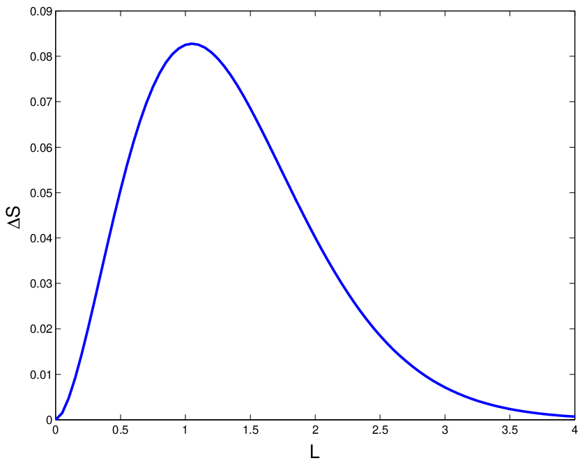
Using the above, it is possible to calculate the entropy of entanglement between the qubit and the angular degree of freedom, and compare it to the total entanglement between the qubit and the two oscillators. Figure 8 shows the difference, $\Delta S$, between these two entanglements. $\Delta S$ asymptotes to zero, such that in the strong coupling regime, the qubit becomes disentangled from the radial degree of freedom and is solely entangled with the angular degree of freedom, as predicted by Eq.(42). Furthermore, this entanglement is maximal. Note that $\Delta S$ is relatively small implying that qubit-oscillators entanglement is concentrated between the angular degree of freedom and the qubit.

The two orthogonal degenerate ground states, $|\Psi\rangle$, and it’s complex conjugate, $|\Psi^{*}\rangle$ from the ansatz Eq. (32), are the two sole ground states where the angular degree of freedom can be treated analogous to a qubit. In any superposition of these two states, the states of the angular degree of freedom is in the subspace spanned by the states $\mathcal{U}_{m}(\phi)$ with $m=0,\pm 1$ - now a three-level system, or qutrit.

As shown in figure 5, for any superposition, the ground state entanglement does not asymptote to the maximal value, but however, there is no ground state superposition that has zero entanglement, as in the single oscillator ($E\otimes\beta$) case. In the large coupling limit, the radial degree of freedom still becomes separable, such that the entanglement is concentrated between the qubit and the angular degree of freedom for all ground possible states. The observation that in all superpositions the angular degree of freedom is viewed as a qutrit rather than a qubit could explain why the entanglement is never zero - as seen in the single oscillator case - nor maximal.

For completeness, we now consider the effect of applying a transverse magnetic field to the qubit, in the direction perpendicular to the oscillator displacements. The Hamiltonian thus becomes

where $\Delta$ is the strength of the magnetic field.

With respect to the fixed point structure in the classical analogue, the addition of the $\Delta$ term has the effect of destroying the stable ring of fixed points, leaving four stable points, at

and

This implies that again a pitchfork bifurcation is present, with the critical coupling, $L^{2}=16\omega^{2}\Delta^{2}$. This should again manifest itself in the large $\Delta$ limit of the entanglement in the ground state, as in the $E\otimes\beta$ model.

Moving to the quantum regime, the ground state is no longer degenerate, and the presence of the transverse field forces the ground state into a maximally entangled state in the large coupling limit.

From figure 9, it’s clear that the bifurcation in the $E\otimes\varepsilon$ model plays a similar role as that in the $E\otimes\beta$ model, in the large $\Delta/\omega$ limit (the classical limit of the oscillator). The gradient of the entropy of entanglement curve with respect to $L$ becomes steeper around the critical point, and we see the division into the “separable” and “entangled” parameter regions.

References

- H.L. Haselgrove, M.A. Nielsen and T.J. Osborne (2003a) H.L. Haselgrove, M.A. Nielsen and T.J. Osborne (2003a), eprint quant-ph/0303022.
- J.I. Latorre, E. Rico and G. Vidal (2003) J.I. Latorre, E. Rico and G. Vidal (2003), eprint quant-ph/0304098.
- T.A. Costi and R.H. McKenzie (2003) T.A. Costi and R.H. McKenzie, Phys. Rev. A 68, 034301 (2003).
- A.P. Hines, R.H. McKenzie and G.J. Milburn (2003) A.P. Hines, R.H. McKenzie and G.J. Milburn, Phys. Rev. A 67, 013609 (2003).
- A. Osterloh, L. Amico, G. Falci and R. Fazio (2002) A. Osterloh, L. Amico, G. Falci and R. Fazio, Nature 416, 608 (2002).
- T.J. Osborne and M.A. Nielsen (2002) T.J. Osborne and M.A. Nielsen, Phys. Rev. A 66, 032110 (2002).
- D. Gunlycke, S. Bose, V.M. Kendon and V. Vedral (2001) D. Gunlycke, S. Bose, V.M. Kendon and V. Vedral, Phys. Rev. A 64, 042302 (2001).
- N. Lambert, C. Emary and T. Brandes (2003) N. Lambert, C. Emary and T. Brandes (2003), eprint quant-ph/0309027.
- H.L. Haselgrove, M.A. Nielsen and T.J. Osborne (2003b) H.L. Haselgrove, M.A. Nielsen and T.J. Osborne (2003b), eprint quant-ph/0308083.
- F. Verstraete, M.A Martín-Delgado and J.I. Cirac (2003) F. Verstraete, M.A Martín-Delgado and J.I. Cirac (2003), to be published in Physical Review Letters, eprint quant-ph/0311087.
- G. Vidal, J.I. Latorre, E. Rico and A. Kitaev (2003) G. Vidal, J.I. Latorre, E. Rico and A. Kitaev, Phys. Rev. Lett 90, 227902 (2003).
- A.J. Leggett, S. Chakravarty, A.T. Dorsey, M.P.A. Fisher, A. Gerg and W. Zwerger (1987) A.J. Leggett, S. Chakravarty, A.T. Dorsey, M.P.A. Fisher, A. Gerg and W. Zwerger, Rev. Mod. Phys. 59, 1 (1987).
- Weiss (1999) U. Weiss, Quantum Dissipative systems (World Scientific, 1999), 2nd ed.
- G. Levine and V.N. Muthukumar (2003) G. Levine and V.N. Muthukumar (2003), eprint cond-mat/0301463.
- Englman (1972) R. Englman, The Jahn-Teller Effect in Molecules and Crystals (John Wiley & Sons Ltd., 1972).
- A.P. Hines, G.J. Milburn and R.H. McKenzie (2003) A.P. Hines, G.J. Milburn and R.H. McKenzie (2003), eprint quant-ph/0308165.
- Sjöqvist (2000) E. Sjöqvist, Int. J. Quantum Chem. 77, 526 (2000).
- C. Emary and T. Brandes (2003) C. Emary and T. Brandes (2003), eprint cond-mat/0301273.
- P. Glendinning (1994) P. Glendinning, Stability, instability and chaos: an introduction to the theory of nonlinear differential equations (Cambridge University Press, 1994).
- G.D. Mahan (1990) G.D. Mahan, Many-particle physics (Plenum Press, New York, 1990), 2nd ed.
- H. Yamasaki, Y. Natsume, A. Terai and H Nakamura (2003) H. Yamasaki, Y. Natsume, A. Terai and H Nakamura (2003), eprint cond-mat/0304484.
- Englman (1962) R. Englman, Phys. Letters 2, 228 (1962).
- C. Monroe, D.M. Meekhof, B.E. King, W.M. Itano and D.J. Wineland (1995) C. Monroe, D.M. Meekhof, B.E. King, W.M. Itano and D.J. Wineland, Phys. Rev. Lett. 75, 4714 (1995).
- S. Hill and W.K. Wooters (1997) S. Hill and W.K. Wooters, Phys. Rev. Lett. 108, 171 (1997).
- W.K. Wooters (2001) W.K. Wooters, Q. Inf. Comp. 1, 27 (2001).
- J. Steinbach, J. Twamley, and P. L. Knight (1997) J. Steinbach, J. Twamley, and P. L. Knight, Phys. Rev. A 56, 4815 (1997).
- Mead (1992) C. A. Mead, Rev. Mod. Phys. 64, 51 (1992).
- J.E. Han and O. Gunnarsson (2000) J.E. Han and O. Gunnarsson, Physica B 292, 196 (2000).
- C.M. Caves, K.S. Thorne, R.W.P. Drever, V.D. Sandberg and M. Zimmermann (1980) C.M. Caves, K.S. Thorne, R.W.P. Drever, V.D. Sandberg and M. Zimmermann, Rev. Mod. Phys. 52, 342 (1980).