Algorithmic Cooling of Spins: A Practicable Method for Increasing Polarization
An efficient technique to generate ensembles of spins that are highly polarized by external magnetic fields is the Holy Grail in Nuclear Magnetic Resonance (NMR) spectroscopy. Since spin-half nuclei have steady-state polarization biases that increase inversely with temperature, spins exhibiting high polarization biases are considered cool, even when their environment is warm. Existing spin-cooling techniques [1, 2, 3, 4] are highly limited in their efficiency and usefulness. Algorithmic cooling [5] is a promising new spin-cooling approach that employs data compression methods in open systems. It reduces the entropy of spins on long molecules to a point far beyond Shannon’s bound on reversible entropy manipulations (an information-theoretic version of the 2nd Law of Thermodynamics), thus increasing their polarization. Here we present an efficient and experimentally feasible algorithmic cooling technique that cools spins to very low temperatures even on short molecules. This practicable algorithmic cooling could lead to breakthroughs in high-sensitivity NMR spectroscopy in the near future, and to the development of scalable NMR quantum computers in the far future. Moreover, while the cooling algorithm itself is classical, it uses quantum gates in its implementation, thus representing the first short-term application of quantum computing devices.
NMR is a technique used for studying nuclear spins in magnetic fields [6]. NMR techniques are extremely useful in identifying and characterizing chemical materials, potentially including materials that appear at negligible levels. There are numerous NMR applications in biology, medicine, chemistry, and physics, for instance magnetic resonance imaging (used for identifying malfunctions of various body organs, for monitoring brain activities, etc.), identifying materials (such as explosives or narcotics) for security purposes, monitoring the purity of materials, and much more. A major challenge in the application of NMR techniques is to overcome difficulties related to the Signal-to-Noise Ratio (SNR). Several potential methods have been proposed for improving the SNR, but each of them has its problems and limitations. We thoroughly review in the Supplementary Information A the six main existing solutions to the SNR problem. In brief, the first (and not very effective) three methods involve cooling the entire system, increasing the magnetic field, and increasing the sample size. The fourth method involves repeated sampling over time, a very feasible and commonly practised solution to the SNR problem. Its limitation is that in order to improve the SNR by a factor of , spectroscopy requires repetitions, making it an overly costly and time-consuming method.
The fifth and sixth methods for improving the SNR provide ways for cooling the spins without cooling the environment, which in this case refers to the molecules’ degrees of freedom. This approach, known as “effective cooling” of the spins [1, 2, 3], is at the core of this current work, and is explained in more detail in Supplementary Information A. The spins cooled by the effective cooling can be used for spectroscopy as long as they have not relaxed back to their thermal equilibrium state. For two-level systems the connection between the temperature, the entropy, and the population probability is a simple one. The population difference between these two levels is known as the polarization bias. Consider a single spin-half particle in a constant magnetic field. At equilibrium with a thermal heat bath the probability of this spin to be up or down (i.e. parallel or anti-parallel to the field’s direction) is given by: , and . The polarization bias, , is around — in conventional NMR systems, so all the following calculations are done to leading order in . A spin temperature at equilibrium is . A single spin can be viewed as a single bit with “0” meaning spin-up and “1” meaning spin-down, and thus, the single spin (Shannon’s) entropy is . A spin temperature out of thermal equilibrium is still defined via the same formulas. Therefore, when a system is removed from thermal equilibrium, increasing the spins’ polarization bias is equivalent to cooling the spins (without cooling the system) and to decreasing their entropy.
One of these latter two methods for effective cooling of the spins is the reversible polarization compression (RPC). It is based on entropy manipulation techniques (very similar to data compression), and can be used to cool some spins (bits) while heating others [2, 3]. Contrary to conventional data compression, RPC techniques focus on the low-entropy bits (spins), namely those that get colder during the entropy manipulation process. The other effective cooling method is known as polarization transfer [1]: If at thermal equilibrium at a given temperature, the spins we want to use for spectroscopy (namely, the observed spins) are less polarized than other spins (namely, auxiliary spins), then transfering polarization from the auxiliary highly polarized spins into the observed spins is equivalent to cooling the observed spins, while heating the auxiliary spins. In its most general form the RPC can be applied to spins which have different initial polarization biases. It follows that polarization transfer is merely a special case of RPC. Therefore, we refer to these two techniques together as RPC.
RPC can be understood as reversible, in-place, lossless, adiabatic entropy manipulations in a closed system. Unfortunately, as in data compression, RPC techniques are limited in their cooling applicability because Shannon’s bound states that entropy in the closed system cannot decrease. [Shannon’s bound on entropy manipulations is an information-theoretic version of the 2nd Law of Thermodynamics.] Polarization transfer is limited because the increase of the polarization bias is bounded by the spin polarization bias of the auxiliary highly-polarized spins. RPC done on uncorrelated spins with equal biases requires extremely long molecules in order to provide significant cooling. The total entropy of such spins satisfies . Therefore, with for instance, molecules of length of an order of magnitude of are required in order to cool a single spin close to zero temperature. For more modest (but still significant) cooling, one can use smaller molecules (with ) and compress the entropy into fully-random spins. The entropy of the remaining single spin satisfies , thus we can at most improve its polarization to
| (1) |
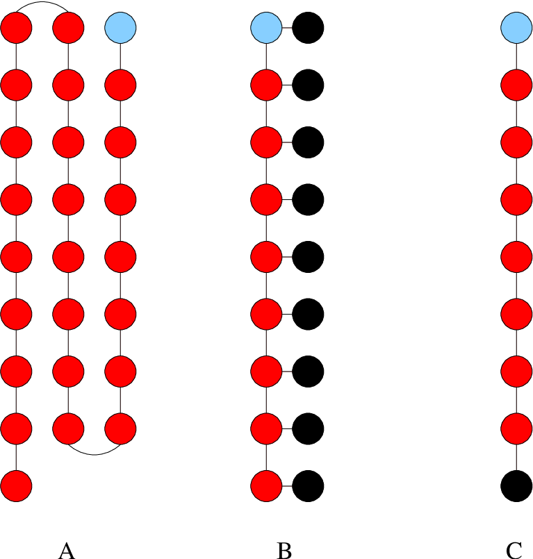
Figure 1A provides an illustration of how Shannon’s bound limits RPC techniques. Unfortunately, manipulating many spins, say , is a very difficult task, and the gain of in polarization here is not nearly substantial enough to justify putting this technique into practice.
We and our colleagues (Boykin, Mor, Roychowdhury, Vatan and Vrijen, hereinafter refered to as BMRVV), invented a promising new spin-cooling technique which we call Algorithmic cooling [5]. Algorithmic cooling expands the effective cooling techniques much further by exploiting entropy manipulations in open systems. It combines RPC with relaxation (namely, thermalization) of the hotter spins, as a way of pumping entropy outside the system and cooling the system much beyond Shannon’s bound. In order to pump the entropy out of the system, algorithmic cooling employs regular spins (which we call computation spins) together with rapidly relaxing spins. Rapidly relaxing spins are auxiliary spins that return to their thermal equilibrium state very rapidly. We refer to these spins as reset spins, or, equivalently, reset bits. The ratio, , between the relaxation time of the computation spins and the relaxation time of the reset spins must satisfy . This is vital if we wish to perform many cooling steps on the system.
The BMRVV algorithmic cooling used blocks of computation bits and pushed cooled spins to one end of such blocks in the molecule. To obtain significant cooling, the algorithm required very long molecules of hundreds or even thousands of spins, because its analysis relied on the law of large numbers. As a result, although much better than any RPC technique, the BMRVV algorithmic cooling was still far from having any practical implications.
In order to overcome the need for large molecules, and at the same time capitalize on the great advantages offered by algorithmic cooling, we searched for new types of algorithms that would not necessitate the use of the law of large numbers for their analysis. Here we present examples of a novel, efficient, and experimentally feasible algorithmic cooling technique which we name “practicable algorithmic cooling”. The space requirements of practicable algorithmic cooling are much improved relative to the RPC, as we illustrate in Figures 1B and 1C. In contrast to the BMRVV algorithm, practicable algorithmic cooling techniques determine in advance the polarization bias of each cooled spin at each step of the algorithm. We therefore do not need to make use of the law of large numbers in the analysis of these techniques, thus bypassing the shortcomings of the BMRVV algorithmic cooling. Practicable algorithmic cooling allows the use of very short molecules to achieve the same level of cooling as the BMRVV achieves using much longer molecules, e.g., 34 spins instead of 180 spins, as we demonstrate explicitly in Supplementary Information B.
Both RPC and algorithmic cooling can be understood as applying a set of logical gates, such as NOT, SWAP etc., onto the bits. For instance, one simple way to obtain polarization transfer is by a SWAP gate. In reality, spins correspond to quantum bits. Here we provide a simplified “classical” explanation, and the more complete “quantum” explanation is provided in Supplementary Information C. A molecule with spins can represent an -bit computing device. A macroscopic number of identical molecules is available in a bulk system, and these molecules act as though they are many computers performing the same computation in parallel. To perform a desired computation, the same sequence of external pulses is applied to all the molecules/computers.
Algorithmic cooling is based on combining three very different operations:
- 1.
RPC steps change the (local) entropy in the system so that some computation bits are cooled while other computation bits become much hotter than the environment.
- 2.
Controlled interactions allow the hotter computation bits to adiabatically lose their entropy to a set of reset bits via polarization transfer from the reset bits into these specific computation bits.
- 3.
The reset bits rapidly return to their initial conditions and convey their entropy to the environment, while the colder parts (the computation bits) remain isolated, so that the entire system is cooled.
By repeatedly alternating between these operations, and by applying a recursive algorithm, spin systems can be cooled to very low temperatures.
In our simplest practicable algorithm there is an array of computation bits, and each computation bit has a neighbouring reset bit with which it can be swapped. The algorithm uses polarization transfer steps, reset steps and the 3-bit RPC step which we call 3-bit-compression (3B-Comp). The 3B-Comp can be built, for instance, via the following two gates: 1.—Use bit as a control, and bit as a target; apply a CNOT (Controlled-NOT) operation: , , where denotes a logical eXclusive OR (XOR). 2.—Use bit B as a control, and bits A and C as targets; apply a variant of a C-SWAP operation: , , ; this means that and are swapped if . The effect of a 3B-Comp step in case it is applied onto three bits with equal bias is to increase the bias of bit to
| (2) |
See Supplementary Information D for calculation details. A simplified example for practicable algorithmic cooling based on these three steps and using computation bits is presented in Figure 2.
In many realistic cases the polarization bias of the reset bits at thermal equilibrium is higher than the polarization bias of the computation bits. By performing an initiation process of polarization transfer from relevant reset bits to relevant computation bits, prior to any polarization compression, we cool the computation bits to the initial bias of the reset bits, , the zero’th purification level. See for instance Figure 3.
In the algorithm we now present, we attempt to cool a single bit much more rapidly than possible in the reversible processes. In order to cool a single bit (say, bit ) to the first purification level, , start with three computation bits, , perform a Polarization Transfer (PT) step to initiate them, and perform 3B-Comp to increase the polarization of bit . In order to cool one bit (say, bit ) to the second purification level (polarization bias ), start with 5 computation bits . Perform a PT step in parallel to initiate bits , followed by a 3B-Comp that cools to a bias . Then repeat the above (PT + 3B-Comp) on bits to cool bit , and then on bits to cool bit as well. Finally, apply 3B-Comp to bits to purify bit to the second purification level , which for small biases gives .
This (very simple) practicable algorithmic cooling, which uses the 3B-Comp, PT, and RESET steps, is now easily generalized to cool a single spin to any purification level . Let be an index telling the polarization level . To obtain one bit at a purification level we define the procedure . Let be the PT step from a reset bit to bit to yield a polarization bias . Then the procedure contains three such PT steps (performed in parallel on three neighbouring bits) followed by one 3B-Comp that cools the left bit (among the three) to level 1. In order to keep track of the locations of the cooled bit we mention here the location of the cooled bit. For an array of bits, we write to say that is applied on the three bits so that bit is cooled to a bias level 1. Similarly, means that is applied on the five bits , so that bit is cooled to a bias level . We use the notation to present the 3B-Comp applied onto bits , purifying bit from to . Then, the full algorithm has a simple recursive form: for
| (3) |
applied from right to left ( is applied first). For instance, is the 3B-Comp applied after reset. The procedure cooling one bit to the second level (starting with five bits) is written as . Clearly, can be applied to any , can be applied to any , and can be applied to any . Thus, if we wish to bring a single bit to a polarization level , then computation bits and reset bits are required. We conclude that the algorithm uses
| (4) |
bits. Due to Eq.( 2) the final polarization bias is , as long as .
Let us now calculate the time complexity of the algorithm. The number of time steps in operation presented above is with , (since the three resets are done in parallel), , and , for any . The recursive formula yields , so that finally
| (5) |
If we count the reset steps only, assuming a much longer time for reset steps than for the other steps, then we get reset time steps. In Supplementary Information B we compare the space and time complexity of this practicable algorithmic cooling with the BMRVV algorithmic cooling.
If we use the reset bits also for the computation, we can improve the space complexity by a factor of 2. The algorithm then uses computation bits and one reset bit, thus a total of bits. See Supplementary Information E for a full description of this algorithm. In Figure 1 we compare the two algorithms descibed here with the RPC, to explicitly illustrate the advantages of practicable algorithmic cooling.
We suggested here an algorithmic cooling technique which is feasible with existing technology. A variant of the 3B-Comp step was implemented by [9] following Schulman and Vazirani’s RPC (their molecular-scale heat engine) [3]. The PT plus RESET steps have been implemented by us and our colleagues [7, 8] following the theoretical ideas presented in this current work. Thus, all steps needed for implementing practicable algorithmic cooling of spins have already been successfully implemented in NMR laboratories. Both these implementations use Carbon molecules that contain two enriched atoms which have spin-half nuclei. In addition to the Carbons, the 3B-Comp experiment [9] also uses one Bromine nucleus, the 3-bit molecule being . The compression yields a single cooled bit with a polarization bias increased by a factor of 1.25. The experimental PT and RESET steps [7, 8] use one Hydrogen and the two Carbons, and the 3-bit molecule is the Trichloroethylene (TCE) molecule (see Figure 3), with the two Carbons being the computation bits and the Hydrogen being the reset bit. This work of [7, 8] implements our ideas in order to prove experimentally that it is possible to bypass Shannon’s bound on entropy manipulations. It is important to note that cooling spins to high purification levels is a feasible task but certainly not an easy one. Addressing specific spins in molecules containing many spins is a very challenging operation from an experimental point of view. Another important challenge is achieving a sufficiently good ratio that will allow the performance of many reset operations, before the cooled bits naturally re-thermalize.
As demonstrated here the theoretical practicable algorithmic cooling is a purely classical algorithm. However, the building blocks are spin-half particles which are quantum bits, and NMR machine pulses which implement quantum gates, that have no classical analogues. Practicable algorithmic cooling is, therefore, the first short-term application of quantum computing devices(11 1 Practicable algorithmic cooling is also one of the first short-term applications of quantum information processing), using simple quantum computing devices to improve SNR in NMR spectroscopy and imaging. Both practicable algorithmic cooling and quantum key distribution could lead to implement
Algorithmic cooling could also have an important long-term application, namely, quantum computing devices that can run important quantum algorithms such as factorizing large numbers [10]. NMR quantum computers [11, 12] are currently the most successful quantum computing devices (see for instance, [13]), but are known to suffer from severe scalability problems [14, 15, 5]. Impressive theoretical solutions were provided in [3, 5] but only the algorithms presented here can lead to a realistic solution. As explained in Supplementary Information A1, practicable algorithmic cooling can be used for building scalable NMR quantum computers of 20-50 quantum bits if electron spins will be used for the PT and RESET steps.
References
- [1] Morris, G.A. & Freedman, R. Enhancement of nuclear magnetic resonance signals by polarization transfer. J. Am. Chem. Soc. 101, 760–762 (1979).
- [2] Sørensen, O.W. Polarization transfer experiments in high-resolution NMR spectroscopy. Prog. Nuc. Mag. Res. spect. 21, 503–569 (1989).
- [3] Schulman, L.J. & Vazirani, U. Molecular scale heat engines and scalable quantum computation. Proc. 31’st ACM STOC (Symp. Theory of Computing) 322–329 (1999).
- [4] Farrar, C.T., Hall, D.A., Gerfen, G.J., Inati, S.J. & Griffin, R.G. Mechanism of dynamic nuclear polarization in high magnetic fields. J. Chem. Phys. 114, 4922-4933 (2001).
- [5] Boykin, P.O., Mor, T., Roychowdhury, V., Vatan, F. & Vrijen, R. Algorithmic cooling and scalable NMR quantum computers. Proc. Natl. Acad. Sci. 99, 3388–3393 (2002).
- [6] Slichter, C.P. Principles of Magnetic Resonance (Springer-Verlag, 1990).
- [7] Brassard, G., Fernandez, J.M., Laflamme, R., Mor, T. & Weinstein, Y. Experimental cooling of NMR spins beyond Shannon’s bound. manuscript in preparation.
- [8] Weinstein, Y. Quantum Computation and Algorithmic Cooling by Nuclear Magnetic Resonance M.Sc. Thesis (Technion, Haifa, 2003).
- [9] Chang, D.E., Vandersypen, L.M.K. & Steffen, M. NMR implementation of a building block for scalable quantum computation. Chem. Phys. Lett. 338, 337-344 (2001).
- [10] Shor, P. Polynomial-time algorithms for prime factorization and discrete logarithms on a quantum computer. SIAM J. on Comp. 26, 1484–1509 (1997).
- [11] Cory, D.G., Fahmy, A.F. & Havel, T.F. Ensemble quantum computing by NMR spectroscopy. Proc. Natl. Acad. Sci. 94, 1634–1639 (1997).
- [12] Gershenfeld, N.A. & Chuang, I.L. Bulk spin-resonance quantum computation. Science 275, 350–356 (1997).
- [13] Vandersypen, L.M.K. et al. Experimental realization of Shor’s quantum factoring algorithm using nuclear magnetic resonance. Nature 414, 883-887 (2001).
- [14] Warren, W.S. The usefulness of NMR quantum computing. Science 277, 1688–1689 (1997).
- [15] DiVincenzo, D.P. Real and realistic quantum computers. Nature 393, 113–114 (1998).
Acknowledgements:
We would like to thank Ilana Frank for very thorough editing of this paper, and to thank Gilles Brassard, Ilana Frank, and Yossi Weinstein for many helpful comments and discussions. T.M. thanks the Israeli Ministry of Defense for supporting a large part of this research. His research was also supported in part by the promotion of research at the Technion, and by the Institute for Future Defense Research. This research was done while J.M.F. was at the Université de Montréal.
Competing interests and materials request statements:
Practicable algorithmic cooling has led to a patent application, US number 60/389,208.
Correspondance and requests for material should be addressed to José M. Fernandez. Email:jose.fernandez@polymtl.ca.


Supplementary Material
Appendix A Solutions to the SNR problem and their limitations
There are several methods which provide rather trivial solutions to the SNR problem. The first of these involves simply cooling the entire system, including cooling the spins, thereby improving the SNR. This is not usually a useful solution because cooling the system can result in modifying the inspected molecules (e.g., solidifying the material), or destroying the sample (e.g., killing the patient). A second method involves increasing the magnetic field, which in some sense is equivalent to cooling the system. This solution is generally much too expensive to be considered feasible, as it adds tremendously to the cost of the necessary machinery. The third method involves increasing the sample size, such as taking a larger blood sample. It is usually impossible, however, to implement this solution due to the large sample size that would be required in order to improve the SNR. One would need to increase the sample size by a factor of in order to improve the SNR by a factor of . In the case of a blood sample, then, to obtain a one hundredfold improvement in SNR one would need to take 100,000 ml. of blood instead of 10 ml., which is clearly not feasible. In some cases increasing the sample size is strictly impossible, for example if the sample in question is a human brain. NMR machine size limitations also severely limit the applicability of this method. The fourth method involves repeated sampling over time. This is a very feasible and commonly practised solution to the SNR problem. Its limitation is that in order to improve the SNR by a factor of , spectroscopy requires repetitions, making it an overly costly and time consuming method. In many cases it is also simply impractical, due to changes over time in the sample during the spectroscopy process (e.g., changes in concentration of a material in a certain body organ). The long recovery time between measurements also contributes to the impracticality of this method. Furthermore, this solution is less useful if the noise in question is not a Gaussian noise.
An additional two methods provide ways for cooling the spins without cooling the environment, which in this case refers to the molecules’ degrees of freedom. This approach is known as “effective cooling” of the spins. Such cooling is as good as regular cooling of the system, because the cooled spins can be used for spectroscopy as long as they have not relaxed back to their thermal equilibrium state. For k-level quantum systems there is, generally, a complex relationship between temperature, entropy, and population density at the different levels. For the sake of simplicity we shall focus here only on two-level systems, namely spin-half particles. Note, however, that the results here can be generalized also to higher level systems, and to quantum systems other than spins. For two-level systems the connection between the temperature, the entropy, and the population density is a simple one. In two-level systems the population density difference is known as the polarization bias. Cooling the system and therefore also the spins (after they reach thermal equilibrium) results in increasing the spins’ polarization bias, and decreasing their entropy. Consider a single spin in a constant magnetic field. At equilibrium with a thermal heat bath the probability of this spin to be up or down (i.e. parallel or anti-parallel to the field’s direction) is given by: , and . The polarization bias, , is calculated to be , where is the energy gap between the up and down states of the spin, is Boltzman’s coefficient and is the temperature of the thermal heat bath. Note that with the magnetic field, and the material dependant gyromagnetic constant which depends on the nucleus or particle, and is thus responsible for causing the differences in polarization biases [the 13Carbon’s nucleus, for instance, is 4 times more polarized than Hydrogen’s nucleus; electron-spin is about times more polarized than Hydrogen’s nucleus.] For high temperatures or small biases we approximate
| (6) |
to leading order. A spin temperature at equilibrium is therefore , which is to leading order (for small ). A single spin can be viewed as a single bit with “0” meaning spin-up and “1” meaning spin-down. Then, the single spin entropy (for a small polarization bias) is
| (7) |
A spin temperature out of thermal equilibrium is still defined via the same formulas. Therefore, when a system is removed from thermal equilibrium, increasing the spins’ polarization bias is equivalent to cooling the spins (without cooling the system) and to decreasing their entropy. What we have learned about single spins can be generalized to several spins on a single molecule.
One method for effective cooling of the spins is the reversible polarization compression (RPC). As is explained in the paper, RPC techniques essentially involve harnessing the powerful data compression tools which have been developed over the past several decades and making use of them to cool spins, as much as is allowed by Shannon’s bound on entropy manipulations in a closed system [3]. Let us present in more details the example of how Shannon’s bound limits RPC techniques. The total entropy of the uncorrelated spins with equal biases satisfies . This entropy could be compressed into high entropy spins, leaving extremely cold spins that have almost zero entropy. Due to the preservation of entropy, the number of extremely cold bits cannot exceed . With for instance, extremely long molecules whose length is of an order of magnitude of are required in order to cool a single spin close to zero temperature. If we use smaller molecules, with , and we compress the entropy into fully-random spins, the entropy of the remaining single spin satisfies . Thus we can at most reduce its entropy to , so that its polarization bias is improved to
| (8) |
Unfortunately, manipulating many spins, say , is a very difficult task, and the gain of in polarization here is not nearly substantial enough to justify putting this technique into practice. It is interesting to note that improving the SNR by a factor of can either be performed using spins via RPC, or using repetitions via repeated sampling over time, or using samples at once, via increasing the sample size times .
The other effective cooling method is the special case of RPC called Polarization transfer. Polarization transfer is limited as a cooling technique because the increase of the polarization bias of the observed spins is bounded by the spin polarization bias of the highly polarized auxiliary spins. The polarization transfer method is commonly implemented by transfering the polarization among nuclear spins on the same molecule. This form of implementation is regularly used in NMR spectroscopy, and it provides, say, an increase of about one order of magnitude. As a simple demostration, consider for example, the 3-bit molecule trichloroethylene (TCE) shown in Figure 3 in the paper. The Hydrogen’s nucleus is four times more polarized than each of the Carbons’ nuclei, and can be used via polarization transfer to cool a single Carbon (say, the Carbon reffered to as C2), by a factor of four.
A different form of polarization transfer involves removing entropy from the nuclear spins into electron spins or into other molecules. This technique is still at initial stages of its developement [4], but might become extremely important in the future as is explained in the Discussion of the paper and in Appendix A.1.
A.1 Polarization transfer with electron spins
Suppose that performing polarization transfer with spins other than the nuclear spins on the same molecule (e.g., spins on other types of molecules, or electron spins on the same molecule) were to become feasible. It would clearly open interesting options potentially leading to a much more impressive effective cooling than the regular polarization transfer onto neighboring nuclear spins. Polarization transfer with electron spins [4] could lead to three and maybe even four orders of magnitude of polarization increase. Unfortunately, severe technical difficulties with the implementation of this method, such as the need to master two very different electromagnetic frequencies within one machine, have so far prevented it from being adopted as a common practice. However, if such polarization transfer steps come into practice, and if the same machinery were to allow conventional NMR techniques as well, then algorithmic cooling could be applied with much better parameters. First, could be increased to around or even . Second, the ratio could easily reach or maybe even . With these numbers, scalable quantum computers of 20-50 bits might become feasible, as can be seen in the tables presented in Appendix B.
Appendix B Comparison with the original algorithmic cooling
In order to compare our practicable algorithmic cooling algorithms with the BMRVV algorithmic cooling we need to consider longer molecules, and more time steps than considered in the text. This clearly makes the schemes unfeasible with existing technology. However, if such parameters become feasible, for instance using the techniques described in Appendix A.1, then medium-scale quantum computing devices of size 20-50 quantum bits can be built. It is important to mention that a comparison of the BMRVV algorithmic cooling with algorithims for RPC is provided in the supplementary material (Appendix C) of [5], to clearly show the advantage of the BMRVV algorithmic cooling over RPC.
In the following, we use the structure in which there are computation bits and a reset bit attached to each computation bit. For any desired final number of cooled bits , the algorithm described in the text, namely PAC1 (Practicable Algorithmic Cooling 1), requires computation bits, and the number of total time steps is . These numbers are obtained as trivial generalizations of Eq. 4 and 5 in the paper. We compare the performance of our new algorithmic cooling and the BMRVV algorithmic cooling [5] in a case where the goal is to obtain 20 extremely cold bits.
To obtain 20 cooled bits via Practicable Algorithmic Cooling 1 (PAC1) we need to use computation bits and time steps This can be compared with [5] where [Eq.(9), with ] and [Eq.(10), with ]. However, the required of [5] is different from the required of the current work, because in [5] while here (see Eq 2 in the paper). As a result, a smaller is required in the algorithm of [5], if a similar desired polarization bias is to be obtained. Tables 1 and 2 present a fair comparison between the time-space requirements of the original and the new algorithms. As can be seen, the improvement obtained by our practicable algorithmic cooling (PAC1) is very impressive, both in space and in time.
| 3 | 140 | 25 | ||
| 4 | 180 | 125 |
| 5 | 30 | 4040 | ||
| 7 | 34 | 36440 |
Appendix C Quantum bits and quantum gates in NMR quantum computing
Although here we use the language of classical bits, spins are actually quantum systems, and spin-half particles (two-level systems) are called quantum bits (qubits). A molecule with spin-half nuclei can represent an -qubit computing device. The quantum computing device in this case is actually an ensemble of many such molecules. In ensemble NMR quantum computing [11, 12] each computer is represented by a single molecule, such as the TCE molecule of Figure 3, and the qubits of the computer are represented by the nuclear spins. A macroscopic number of identical molecules is available in a bulk system, and these molecules act as though they are many computers performing the same computation in parallel. The collection of many such molecules is put in a constant magnetic field, so that a small majority of the spins (that represent a single qubit) are aligned with the direction of that field. To perform a desired computation, the same sequence of external pulses is applied to all the molecules/computers. Finally, a measurement of the state of a single qubit is performed by summing over all computers/molecules to read out the output on a particular qubit on all computers. In practicable algorithmic cooling we know in advance the polarization bias of the cooled bits after each step. In BMRVV algorithmic cooling we could also calculate the polarization bias, but it becomes a very cumbersome process. Thus, due to the complexity of the algorithm, the law of large numbers is used, and calculation of the polarization bias is done only after some particular steps called CUT in [5].
For most purposes of this current theoretical work, the gates we consider are classical, and the spins can therefore be considered as classical bits. Only in a lab, the classical gates are implemented via the available quantum gates. Then, the spins must be considered as qubits and the entire process is a simple quantum computing algorithm. However, unlike in other popular quantum algorithms, the use of quantum gates will not produce here any significant speed-up.
Appendix D Details of new bias calculations
as we have seen, the 3B-Comp can be built, for instance, via the following two gates:
- 1.
Use bit as a control, and bit as a target; apply a CNOT (Controlled-NOT) operation: , , where denotes a logical eXlusive OR (XOR).
- 2.
Use bit B as a control, and bits A and C as targets; apply a variant of a C-SWAP operation: , , ; this means that and are swapped if .
The effect of a 3B-Comp step in case it is applied onto three bits with equal bias is as follows:
- •
if after the CNOT operation, the bias of at that stage is (this is the probability of given , all these calculated prior to the CNOT operation; in other words, this is the probability of bit being 0, given that bit is 0 after the CNOT). Due to the CSWAP this bias is transfered to bit ;
- •
if after the CNOT operation, the bias of is still after the CSWAP.
The new bias, , is the weighted average of the two possible biases which is , which gives
| (9) |
for small .
The following single operation can replace the CNOT+CSWAP, performing a 3B-Comp, to cool bit (the heated bits are not in the same state as for the previous 3B-Comp, though):
Note that reset bits can be used for the computation as well. Thus the simplest algorithmic cooling can be obtained via 2 computing bits and one reset bit.
Note also that the strong tools of data compression can easily be used to significantly improve the algorithms, for the price of dealing with more complicated gates.
Appendix E A more space-efficient practicable algorithmic cooling
We consider here the case in which steps 1 and 2 (the 3B-Comp and PT steps) in the outline of algorithmic cooling are combined into one generalized step of RPC. Then, the logical gates are applied onto all bits in the system, that is computation and reset bits, to push the entropy into the reset bits. For comparison with the RPC and PAC1 (see Figure 1) we consider the cooling of a single bit.
Once we use the reset bits for the compression steps as well, replacing the 3B-Comp+PT steps by a generalized RPC, we can much improve the space complexity of the algorithm relative to PAC1. We call this improved algorithm PAC2.
Whenever we used bits in PAC1, namely computation bits, each one having a reset bit as a neighbour, we can now use exactly bits, namely computation bits plus one reset bit. Let us explicitly show how this is done. Let be the polarization bias of the reset bit. In order to cool a single bit, say bit , to start with two computation bits, and one reset bit, , perform PT() followed by PT( to initiate bit , RESET() (by waiting), then perform PT() to initiate bit , and another RESET(). If the thermalization time of the compuation bits is sufficiently large, we now have three bits with polarization bias . Now perform 3B-Comp to increase the polarization of bit .
In order to cool one bit (say, bit ) to the second purification level (polariation bias ), start with 4 computation bits , and one reset bit . Perform PT steps sequentially (with RESET() when needed) to initiate bits , followed by a 3B-Comp on bits that cools bit to a bias . Then, perform PT steps sequentially (with RESET() when needed) to initiate bits , followed by a 3B-Comp on bits that cools bit to a bias . Next, perform PT steps sequentially (with RESET() when needed) to initiate bits , followed by RESET(), and then followed by a 3B-Comp on bits that cools bit to a bias . Finally, apply 3B-Comp to bits to purify bit to the second purification level . Clearly, the same strategy can be used to cool a single bit to using computation bits and a single reset bit. The total space complexity is therefore
| (10) |
Note that which is slightly larger than 5, leading immediately to the numbers presented in Figure 1. Cooling by a factor of 25 requires 17 spins here, while it requires 625 spins in RPC, or it requires repeating the experiment 625 times if no cooling is used.
We should mention, though, that the timing considerations for PAC2 are more demanding than the timing consideartions for PAC2 due to the need of many more SWAP gates. All the steps of the algorithm must be done within the relaxation time of the computation bits, and even more demanding, within the dephasing time (known as ) of the computation bits.