Minimal assumption derivation of a Bell-type inequality
Abstract
John Bell showed that a big class of local hidden-variable models stands in conflict with quantum mechanics and experiment. Recently, there were suggestions that empirical adequate hidden-variable models might exist, which presuppose a weaker notion of local causality. We will show that a Bell-type inequality can be derived also from these weaker assumptions.
Keywords:
Bell’s inequality, common causespacs
03.65.UdI Introduction
The violation of Bell’s inequality by the outcome of an EPR-type spin experiment Einstein et al. 1935; Bohm 1951 seems to exclude a local theory with hidden variables. The underlying reductio ad absurdum proof infers on the grounds of the empirical falsification of the derived inequality that at least one of the required assumptions must be false. The force of the argument requires that the derivation be deductive and that all assumptions be explicit. We aim to extract a minimal set of assumptions needed for a deductive derivation of Bell’s inequalities given perfect correlation of outcomes of an EPR-type spin experiment with parallel settings.
One of the assumptions in Bell’s original derivation Bell 1964 was determinism. Later, he succeeded in deriving a similar inequality without determinism Bell 1971, placing in its stead an assumption later dubbed local causality Bell 1975. As Bell stressed, the notion of local causality he and others used might be challenged. In Hofer-Szabó et al. 1999 it was pointed out, that Reichenbach’s Common Cause Principle Reichenbach 1956 indeed suggests a weaker form of local causality. We will prove here, however, that even from this weaker notion Bell’s inequality can still be derived.11 1 Several of the issues we present in this paper are discussed in more detail in Wüthrich 2004.
II The EPR-Bohm experiment
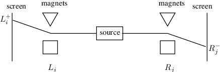
Consider the so-called EPR-Bohm (EPRB) experiment Einstein et al. 1935; Bohm 1951. Two spin- particles in the singlet state
| (1) |
are separated in such a way that one particle moves to a measurement apparatus in the left wing of the experimental setting and the other particle to a measurement apparatus in the right wing (see FIG. 1). The experimenter can choose arbitrarily one of three directions in which the spin is measured with a Stern-Gerlach magnet.
The following terminology follows the reconstruction by Wigner 1970 and which van Fraassen 1989 has subsequently expanded on. The event type22 2 We will speak of event types to distinguish them from the token events which instantiate corresponding event types. that the left (right) measurement apparatus is set to measure the spin in direction is symbolized by (). () symbolizes the event type that the measurement outcome in the left (right) wing of a spin measurement in direction is . There are two possible measurement outcomes spin up () and spin down () for each particle in each direction. The letter will be used like to symbolize directions and like to symbolize measurement outcomes. Formulas in which the variables , , , and appear are meant to hold—if not otherwise stated—for all possible values of the variables. denotes the probability of an event type , which is empirically measurable as the relative frequency of all runs of an EPRB experiment in which the event type is instantiated, with respect to all runs. is the probability of the event type ‘ and ’, measurable as the relative frequency of all runs in which both and are instantiated. is the conditional probability of the event type given the event type , measurable as the relative frequency of instantiations of with respect to the subensemble of all runs in which is instantiated. E.g.
| (2) |
denotes the probability that the measurement outcome is on the left and on the right, when measuring in direction on the left and in direction on the right. These probabilities are predicted by quantum mechanics as
| (3) | ||||
| (4) | ||||
| (5) | ||||
| (6) |
where denotes the angle between the two measurement directions and . Also, the outcomes on each side are predicted separately to be completely random:
| (7) | |||
| (8) |
III Local causality
The derivations of Bell-type inequalities known to us which do not presuppose determinism assume instead what John Bell calls local causality Bell 1975; Clauser and Horne 1974. That is, the assumption that there is common cause variable33 3 For the sake of simplicity, we assume that this partition is discrete and finite. As will become clear in the following, the derivation of Bell’s inequality can also be done without this restriction. which takes on values such that for event types ‘the variable has the value ’ () we have and
| (9) |
Other frequently used names for this condition are factorizability Butterfield 1989 and strong locality Jarrett 1984; Jarrett 1989. It is usually justified by pointing out that it follows from the conjunction of the following three conditions, which are called completeness (equation (10)) and locality (equations (11) and (12)) Jarrett 1984; Jarrett 1989, outcome independence and parameter independence Shimony 1993, or causality and hidden locality van Fraassen 1989:
| (10) | ||||
| (11) | ||||
| (12) |
Equation (10) says that event types or the variable “screens off” and from each other van Fraassen 1989; Butterfield 1989. Van Fraassen van Fraassen 1989 pointed out, that equation (10) can be motivated through Reichenbach’s Principle of Common Cause (PCC) Reichenbach 1956. The principle states, that whenever two different event types and are statistically correlated
| (13) |
and neither is causally relevant for nor for , there exists a common cause variable with values () such that and given are uncorrelated:
| (14) |
In its original formulation the principle is stated only for a common cause
event type , which is included in our formulation as the special case where
can take only two values: , (‘not
’).
The principle was formulated for general common cause variables by
Hofer-Szabó et al. and Placek 2000. Besides the screening-off
condition
Reichenbach 1956 and Hofer-Szabó et al. stipulate further restrictions
on the common cause variable, which are, however, irrelevant for our purposes.
Now, as can be seen from equations (3)-(6), the event type
is in general correlated with event type . It is
| (15) |
and therefore
| (16) |
Supposing that is not causally relevant for and vice versa (which is reinforced by the fact that the setup of the experiment can be chosen so that the instantiations of and in each run of the experiment are space-like separated), PCC requires a common cause variable which fulfills equation (10). There are several different correlations; e.g. is correlated with , and is correlated with . For each of these correlations PCC enforces the consequence that a common cause variable exists. As stressed in Hofer-Szabó et al. 1999 nothing in PCC dictates that the common cause variables of the different correlations have to be the same. However, in all the derivations of Bell’s inequality known to us this identification is made nevertheless. It is further shown in Hofer-Szabó et al. 1999 and Hofer-Szabó et al., that for any set of correlations it is mathematically possible to construct common cause variables. The authors concluded in Hofer-Szabó et al. 1999 that the apparent contradiction between this possibility and the claim that the EPRB correlations do not allow for a common cause variable van Fraassen 1989; Butterfield 1989, is resolved by pointing out that in the derivation of Bell’s inequality a common common cause variable for all measurements is assumed:
“The crucial assumption in the […] derivation of the [Clauser-Horne] inequality is that [the two-valued common cause variable] is a [two-valued common cause variable] for all four correlated pairs, i. e. that [] is a common common cause [variable], shared by different correlations. Without this assumption Bell’s inequality cannot be derived. But there does not seem to be any obvious reason why common causes should also be common common causes, whether of quantum or of any other sort of correlations.” (Italics in the original.)
Showing the mathematical possibility of constructing common cause variables for any set of correlations and in particular for the correlations found in the EPRB experiment is not sufficient for proving the existence of a physically “natural” hidden-variable model for that experiment, however. Besides being common cause variables (thus fulfilling equation (10)), parameter independence should hold, too (equations (11) and (12)). Also, they should not be correlated with the measurement choices. As shown by Szabó Szabó 1998, it is possible to construct a model which fulfills these requirements for each of the common cause variables separately. However, the conjunctions and other logical combinations of the event types that the common cause variables have certain values correlate in that model with the measurement operations. Whether a model can be constructed without these correlations was posed as an open question by Szabó. This question is answered negatively by the derivation of Bell’s inequality that we present in the remainder of this article.
IV Bell’s inequality from separate common causes
IV.1 A weak screening-off principle
Consider an EPRB experiment where the same direction () is chosen in both wings. That is, in each run the event type is instantiated. With this special setting quantum mechanics predicts (see equations (3)-(8), with ) that the measurement outcomes in each wing are random but that the outcomes in one wing are perfectly correlated with the outcomes in the other wing: if and only if the spin of the left particle is up, then the spin of the right particle is down, and vice versa. We refer to this assumption as perfect correlation, or PCORR for short.
Assumption 1 (PCORR)
| (17) |
We use here the definition
| (18) |
Large spatial separation of coinciding events of type and suggests that the respective instances are indeed distinct events. This excludes an explanation of the correlations by event identity, as is the case, for example, with a tossed coin for the perfect correlation of the event types ‘heads up’ and ‘tails down’. Such a perfect correlation is explained in that every instance of ‘heads up’ is also an instance of ‘tails down’, and vice versa. Since the separation is even space-like, no or should be causally relevant for the other. We refer to these two assumptions as separability, SEP for short, and locality 1 (LOC1).
Assumption 2 (SEP)
The coinciding instances of and are distinct events.
Assumption 3 (LOC1)
No or is causally relevant for the other.
Rather, there should be a common cause variable; that is, we assume PCC.
Assumption 4 (PCC)
If two event types and are correlated and the correlation cannot be explained by direct causation nor event identity, then there exists a common cause variable , with values such that and
As already mentioned, we omit the other Reichenbachian conditions Reichenbach 1956; Hofer-Szabó et al. since they are not necessary for our derivation.
This principle together with the assumptions PCORR, SEP and LOC1 implies that there is for each of the EPRB correlations a (separate) common cause variable with .
Result 1
| (19) |
Note that common cause variables can be different for different correlations.
IV.2 Perfect correlation and “determinism”
We now show that from the fact that a perfect correlation is screened off by some variable it follows that without loss of generality the common cause variable can be assumed to be two-valued and that the having of one of the two values of the variables is necessary and sufficient for the instantiation of the two perfectly correlated event types, cf. Suppes and Zanotti 1976.
Let and be perfectly correlated,
and screened-off from each other by a common cause variable,
We can split the set of all values completely into two disjunct subsets, namely in the subset of those values of for which is not zero and in the subset of those for which it is zero:
¿From this definition of it follows already that
| (20) |
i. e. that with is necessary for . Moreover, for all we have by screening off and perfect correlation
| (21) |
That the variable has a value in is a necessary and sufficient condition for . The following calculation shows that with is also necessary and sufficient for .
¿From perfect correlation it follows that
That screens off from yields
Together with the previous equation this implies that is sufficient for for all :
| (22) |
If we have by definition , which implies
By perfect correlation we have therefore also , which in turn implies that
| (23) |
which means that with is also necessary for .
This calculation shows that in the case of a perfect correlation the set of values of the common cause variable decomposes into two relevant sets. This means that whenever there is an (arbitrarily-valued) common cause variable for a perfect correlation, there is also a two-valued common cause variable, namely the disjunction of all event types for which or , respectively.
We refer to as a common cause event type. In the case of a perfect correlation no generality is achieved by allowing for a more than two-valued common cause variable; if there is a common cause variable for a perfect correlation, there is also a common cause event type. Moreover, the common cause event type is a necessary and sufficient condition for the event types that are screened off by it (equations (20), (21), (22) and (23)).
Result 1 thus implies that there is a common cause event type such that
| (24) | |||
| (25) |
The sub- and superscripts of refer to being the common cause event type of and .
The outcome of a spin measurement is always either or and nothing else. We call this assumption exactly one of exactly two possible outcomes (EX).
Assumption 5 (EX)
| (26) | ||||||
| (27) |
As stressed by Fine 1982, among the actual measurements there are always runs in which no outcome is registered, which is normally attributed to the limited efficiency of the detectors and not taken to the statistics. If one assumes instead, that part of these no-outcome runs are caused by the hidden variable, then it is possible to construct empirically adequate models for the EPRB experiments Szabó 2000; Szabó and Fine 2002. With assumption 5, we explicitly exclude such models.
With assumption 5, while is necessary and sufficient for and , its complement, i. e. is necessary and sufficient for the opposite outcomes, i. e. and :
| (28) | |||
| (29) |
IV.3 A minimal theory for spins
In section IV.2 it was found that is sufficient for given parallel settings (), see equation (24). I. e. the conjunction is sufficient for . But because of space-like separation of events of type and that are instantiated in the same run, the latter types should not be causally relevant for the former. The measurement choice in one wing should be causally irrelevant for the outcomes (and the choices) in the other wing. Therefore we should discard from the sufficient conjunction. The part alone is sufficient for . A similar reasoning can be applied to , and , cf. equation (29). This is our assumption locality 2 (LOC2).
Assumption 6 (LOC2)
If is sufficient for , then alone is sufficient for ; and similarly for , i. e. if is sufficient for , then alone is sufficient for .
Moreover, the remaining part is minimally sufficient, in the sense that none of its parts is sufficient on its own.44 4 Minimal sufficient conditions as definied by Graßhoff and May 2001 and Graßhoff and Baumgartner forthcoming. If, for example, is instantiated, but we do not choose to measure , then will not be instantiated. That is to say, we cannot discard yet another conjunct of as we discarded from .
Let us turn to necessary conditions for . To begin with, is necessary: If there is no Stern-Gerlach magnet properly set up () the particle is not deflected either up- or downwards; similarly for , and . Roughly speaking, no outcome without measurement (NOWM).
Assumption 7 (NOWM)
| (30) | ||||||
| (31) |
Second, we saw in section IV.2 that if parallel settings are chosen and is instantiated an event of type does never occur. In other words, implies :
| (32) |
Again we propose a locality condition based on the idea that the measurement choice in one wing should be causally irrelevant for the outcomes (and the choices) in the other wing:55 5 The following version of LOC3 is slightly different from an earlier version of the article. We thank Gabor Hofer-Szabó, Miklos Rédei and Iñaki San Pedro for their comments. If are sufficient for , then alone should be sufficient for . A similar reasoning can be applied to , and , cf. equation (28).
Assumption 8 (LOC3)
If is sufficient for , then alone is sufficient for ; and similarly for , i. e. if is sufficient for , then alone is sufficient for .
By LOC3 it follows from equation (32) that
| (33) |
This is equivalent to
| (34) |
and also to
| (35) |
According to equation (30), is necessary for . That means , but also . Above, we have found (eq. (35)) that . Altogether, this entails , i. e. that is necessary for . Moreover, it is a minimally necessary condition in the sense of Graßhoff and May 2001 since it does not contain any disjuncts. All in all: is a minimally necessary and minimally sufficient condition for . In a similar vein we find that is minimally necessary and minimally sufficient for . We have thus derived in particular the four minimal theories in the sense of Graßhoff and May 2001 as illustrated in FIG. 2.


In a formal notation the four minimal theories read as the following four equations, where is the usual biconditional, which means that the left-hand side implies the right-hand side and vice versa.66 6 For details see Graßhoff and May 2001 and Graßhoff and Baumgartner forthcoming. Note in particular that a correct formal notation of a minimal theory uses what Graßhoff et. al. Graßhoff and May 2001; Graßhoff and Baumgartner forthcoming call a double conditional. This intermediate result is referred to as minimal theories (MTH).
IV.4 No conspiracy
The events of type are not supposed to be influenced by the measuring operations and . One reason for this assumption is that the measurement operations can be chosen arbitrarily before the particles enter the magnetic field of the Stern-Gerlach magnets and that an event of type is assumed to happen before the particles arrive at the magnets. Therefore a causal influence of the measurement operations on events of type would be tantamount to backward causation. Also an inverse statement is supposed to hold: The event types are assumed not to be causally relevant for the measurement operations. This is meant to rule out some kind of “cosmic conspiracy” that whenever an event of type is instantiated, the experimenter would be “forced” to use certain measurement operations. This causal independence between and the measurement operations is assumed to imply the corresponding statistical independence. The same is assumed to hold also for conjunctions of common cause event types. We refer to this condition as no conspiracy (NO-CONS).
Assumption 9 (NO-CONS)
| (39) |
By this condition of statistical independence the three probabilities considered above can be transformed. That is, we have, for instance
The dotted equations are true by definition of conditional probability. In step (i) equation (36) was used. Step (ii) is valid by “no conspiracy” (equation (39)), and (iii) by a theorem of probability calculus, according to which for any and . Transforming the other two expressions in a similar way, we arrive at
| (40) | ||||
| (41) |
| (42) |
Since both terms of the right-hand side of the last equation appear in the sum of the right-hand sides of the first two equations, the following version of the Bell inequality (BELL) follows77 7 It was first derived in this form by Wigner Wigner 1970..
Result 3 (BELL)
| (43) |
This inequality has been empirically falsified, see e. g. Aspect et al. 1982.
The inequality was derived from the following assumptions.
- •
Perfect correlation (PCORR),
- •
separability (SEP),
- •
locality 1 (LOC1),
- •
principle of common cause (PCC),
- •
exactly one of exactly two possible outcomes (EX),
- •
locality 2 (LOC2),
- •
no outcome without measurement (NOWM),
- •
locality 3 (LOC3),
- •
no conspiracy (NO-CONS).
This is a version of Bell’s theorem. It says: If these assumptions are true, the Bell inequality is true. The derivation of the Bell inequality presented here is an improvement on the usual Bell-type arguments, such as Bell 1975 and van Fraassen 1989, in two respects: First, it does not assume a common common cause variable for different correlations. Second, contrary to the usual locality conditions, the ones assumed here do not presuppose a solution to the problems posed by the relation between causal and statistical (in)dependence (see e. g. Spirtes et al. 1993).
V Discussion
Our claim to have presented a minimal assumption derivation of a Bell-type inequality is relative: our set of assumptions is weaker than any set known to us from which a Bell-type inequality can be derived and that contains the assumption of perfect correlation (PCORR). It was one of the achievements of Clauser and Horne 1974 to show that a Bell-type inequality can be derived also if the correlations of outcomes of parallel spin measurements are not assumed to be perfect. Our assumption of correlation is stronger than the one used by Clauser and Horne. However, they assume a common common cause variable for all correlations, which is a stronger assumption than our assumption of possibly different common cause variables for each correlation (PCC). We have not been able to derive a Bell-type inequality without assuming perfect correlation and allowing different common cause variables. If PCORR is indeed a necessary assumption for our derivation of the Bell inequality, it should be possible to construct a model in which PCORR does not hold (being violated by an arbitrary small deviation, say). Since the actually measured correlations are never perfect—a fact that is usually attributed to experimental imperfections—it is not obvious how such a model could be refuted.
Our notion of local causality might be challenged as follows. Even though nothing in PCC dictates that in general the common cause variables of different correlations have to be the same, there might be strong grounds for why they are the same in the context of the EPRB experiment. Indeed, Bell argued for his choice of local causality along the following lines.88 8 For a very good and more detailed discussion of this, see Butterfield 1989. Assume that and are positively correlated. Then
| (44) |
Since coinciding instances of and are space-like separated, neither is causally relevant for the other. Rather, the correlation should be explained by exhibiting some common causes in the overlap of the backward light cones of the coinciding instances. An instance of, say, raises the probability of an instantiation of one of the common causally relevant factors, and this raises the probability of an instantiation of . But given the total state of the overlap of the backward light cones of two coinciding instances, the probability of, say, is assumed to be the same whether is instantiated or not. If the total state of the overlap of the backward light cones is already given, nothing more that could be causally relevant for can be inferred from an instance of .
Along this line of reasoning the total state of the overlap of the backward lightcones99 9 One might argue that the total state of the union of the backward lightcones is a better candidate for a common cause variable Butterfield 1989. The following discussion carries over also to this case. of and is a common cause variable which screens off the correlation:
| (45) |
The common past cannot be altered by choosing one or the other direction for the spin measurement—“facta infecta fieri non possunt” (Placek 2000, p. 185). Therefore the total state of the common past is indeed a common common cause variable for all correlated outcomes, see FIG. 3.

.
This reasoning can be questioned along the following lines. It is reasonable that not all event types that are instantiated in the overlap of the backward light cones of two coinciding instances of the correlated event types are causally relevant for these latter event types. Therefore conditionalizing on the total state is conditionalizing not only on the relevant factors but also on the irrelevant. Moreover, it is conceivable that which event types of the common past are relevant and which are not differs for different measurements. Claiming that the total state of the common past is a common common cause variable, one is thus committed to assume that
“conditionalizing on all other events […] in addition to those affecting [the correlated event types], does not disrupt the stochastic independence induced by conditionalizing on the affecting events.” Butterfield 1989
In particular in the light of Simpson’s paradox Simpson 1951 this assumption has been challenged Cartwright 1979. Here, we will not assess arguments in favour of or against the possibility that conditionalizing on irrelevancies yields unexpected statistical dependencies. Our point is that by weakening the assumption in the way we did, our derivation is conclusive whatever may be the answer to this question.
Acknowledgements.
We would like to thank Guido Bacciagaluppi, Miklós Rédei, Gabor Hofer-Szabó and Iñaki San Pedro for fruitful discussions.References
- Einstein et al. (1935) A. Einstein, B. Podolsky, and N. Rosen, Physical Review 47, 777 (1935).
- Bohm (1951) D. Bohm, Quantum Theory (Prentice Hall, New York, 1951).
- Bell (1964) J. S. Bell, Physics 1, 195 (1964), reprinted in (Bell 1987, p. 14).
- Bell (1971) J. S. Bell, in Foundations of Quantum Mechanics, Proceedings of the International School of Physics ‘Enrico Fermi’ (New York, Academic, 1971), p. 171, reprinted in (Bell 1987, p. 29).
- Bell (1975) J. S. Bell, The theory of local beables, TH-2053-CERN (1975), presented at the Sixth GIFT Seminar, Jaca, 2–7 June 1975, reproduced in Epistemological Letters, March 1976, and reprinted in (Bell 1987, p. 52).
- Hofer-Szabó et al. (1999) G. Hofer-Szabó, M. Rédei, and L. E. Szabó, British Journal for the Philosophy of Science 50, 377 (1999), eprint quant-ph/9805066.
- Reichenbach (1956) H. Reichenbach, The Direction of Time (University of California Press, Los Angeles, 1956).
- Wüthrich (2004) A. Wüthrich, Quantum Correlations and Common Causes (Bern Studies in the History and Philosophy of Science,, 2004).
- Bell (1987) J. S. Bell, Speakable and Unspeakable in Quantum Mechanics (Cambridge University Press, Cambridge, 1987).
- Wigner (1970) E. Wigner, American Journal of Physics 38, 1005 (1970).
- van Fraassen (1989) B. C. van Fraassen, in Cushing and McMullin 1989.
- Clauser and Horne (1974) J. F. Clauser and M. A. Horne, Physical Review D 10, 526 (1974).
- Butterfield (1989) J. Butterfield, in Cushing and McMullin 1989.
- Jarrett (1984) J. P. Jarrett, Noûs 18, 569 (1984).
- Jarrett (1989) J. P. Jarrett, in Cushing and McMullin 1989, pp. 60–79.
- Shimony (1993) A. Shimony, Search for a naturalistic world view, vol. 2 (Cambridge University Press, 1993).
- (17) G. Hofer-Szabó, M. Rédei, and L. E. Szabó, Reichenbachian Common Cause Systems, Forthcoming in International Journal of Theoretical Physics, URL http://philsci-archive.pitt.edu/archive/00001246/.
- Placek (2000) T. Placek, Is Nature determinstic? (Jagiellonian University Press, Kraków, 2000), 1st ed.
- Szabó (1998) L. E. Szabó (1998), eprint quant-ph/9806074.
- Suppes and Zanotti (1976) P. Suppes and M. Zanotti, in Logic and Probability in Quantum Mechanics, edited by P. Suppes (Dordrecht: Reidel, 1976), pp. 445–455.
- Fine (1982) A. Fine, Synthese 50, 279 (1982).
- Szabó (2000) L. Szabó (2000), eprint quant-ph/0002030.
- Szabó and Fine (2002) L. Szabó and A. Fine (2002), URL http://philsci-archive.pitt.edu/archive/00000642/.
- Graßhoff and May (2001) G. Graßhoff and M. May, in Current Issues in Causation, edited by W. Spohn, M. Ledwig, and M. Esfeld (Paderborn: Mentis, 2001), pp. 85–114.
- Graßhoff and Baumgartner (forthcoming) G. Graßhoff and M. Baumgartner, Kausalität und kausales Schliessen (Bern Studies in the History and Philosophy of Science, forthcoming).
- Aspect et al. (1982) A. Aspect, J. Dalibard, and G. Roger, Physical Review Letters 49, 1804 (1982).
- Spirtes et al. (1993) P. Spirtes, C. Glymour, and R. Scheines, Causation, Prediction, and Search (Springer Verlag, 1993).
- Simpson (1951) E. H. Simpson, Journal of the Royal Statistical Society, Ser. B. 13, 238 (1951).
- Cartwright (1979) N. Cartwright, Noûs 13, 419 (1979).
- Cushing and McMullin (1989) J. T. Cushing and E. McMullin, eds., Philosophical Consequences of Quantum Theory. Reflections on Bell’s Theorem (University of Notre Dame Press, Notre Dame, 1989).