An exact effective two-qubit gate in a chain of three spins

Before presenting our main result, we discuss some related works. Our work is motivated by Bose03; Subrahmanyam03 that study quantum state transfer and entanglement distribution in a spin chain of $N$ spins under the free evolution according to the Hamiltonian

where $\vec{\sigma}_{i}\cdot\vec{\sigma}_{j}\equiv\sigma_{\!x\,i}\,\sigma_{\!x\,j}+\sigma_{\!y\,i}\,\sigma_{\!y\,j}+\sigma_{\!z\,i}\,\sigma_{\!z\,j}$. Perfect (near perfect) state transfer between the remotest spins are only allowed for a 4-spin closed (open) chain Bose03, apart from the trivial case of 2 spins.

Our work is also motivated by Cubitt03, which considers a similar $3$-spin chain with only nearest neighbor coupling. They found mixed separable initial states such that the two remote spins become entangled by the Hamiltonian without ever entangling the mediating spin. They also proved that such phenomenon is impossible for pure states. In our system, the mediating spin is entangled during the process, but is completely disentangled from the data qubits at the end, leaving the data qubits maximally entangled.

Our work can also find application in the quantum computation scheme in Benjamin03. Reference Benjamin03 investigated effective gates between non-neighboring spins in a Heisenberg spin chain (3) with untunable couplings. Our result is an analog in the XY model (1), and has the merit of producing a much simpler two-qubit gate (the composition of a swap gate and a controlled-phase gate) compared to Benjamin03.

Time optimal construction of indirect $2$-qubit gates, such as swap or cnot, is considered in Khaneja03. Our approach is different in requiring no local manipulations, and also in obtaining an exact implementation of the gate.

During the initial preparation of our manuscript, related works Christandl03 were reported independently by Christandl et al. They considered perfect quantum state transfer over more general spin networks (besides linear chains) under the same Hamiltonian (1). When the interaction strength is homogeneous, i.e. $\omega_{ij}=\omega$, they found that perfect state transfer is possible only between the two ends of an $N=2$ or $3$ linear chain, or between the antipoles for a hypercube. When the coupling strength can be suitably tuned, perfect state transfer is possible for any linear chain. Extensions to a Heisenberg chain (3) was considered when a tunable, local magnetic field can be applied to each spin. Our motivating scheme in Sec. II.1 coincides with the $N=3$ case of Christandl03, which also motivated some extensions in Sec. III for longer chains. Our work differs in explicitly considering the evolution on all three spins (instead of a subspace relevant to quantum state transfer as considered in Christandl03). We exploit different initial configurations that result in more flexibility and better efficiencies in tasks other than state transfer, beyond immediate implications of the ability to perform state transfer.

The Hamiltonian for our $3$-spin chain (1) is simply

We first motivate our result by considering quantum state transfer, say, from the first to the last spin:

Suppose the initial state of the first spin is $\left|\varphi\right\rangle_{1}=\alpha\left|0\right\rangle_{1}+\beta\left|1\right\rangle_{1}$, where $\left|\alpha\right|^{2}+\left|\beta\right|^{2}=1$. The initial state of the three spins can be written in the form,

The state will evolve, under the Hamiltonian (4), as

where the first term is not affected by the Hamiltonian because $H\left|{000}\right\rangle=0$. The second term can be evaluated analytically. To do this, we make use of the special properties of the raising and lowering operators to obtain

Using (8), the Taylor series expansion can be evaluated explicitly

where $\gamma=\sqrt{\omega^{2}+\lambda^{2}}$. When $\lambda=\omega$ and $t=\tau\equiv\mbox{$\frac{\pi}{\sqrt{2}\omega}$}$, we have

and

Perfect state transfer (5) is then obtained by applying the local unitary operator $\sigma_{\!z\,3}$ to the last spin.

To obtain our key result and to better understand the above scheme, we examine the full matrix representation of the unitary operator $U\equiv\exp(-iH\tau)$, with the basis ordered as $|000\rangle$, $|001\rangle$, $|100\rangle$, $|101\rangle$, $|010\rangle$, $|011\rangle$, $|110\rangle$, $|111\rangle$,

The subspaces spanned by $|0\rangle_{2}$ and $|1\rangle_{2}$ are invariant under $U$. Thus restricting $U$ to either subspace forms an effective two-qubit gate for the remote spins $1$ and $3$. In particular, we can consider the restriction $\tilde{U}$ of $U$ to the “$|0\rangle_{2}$ subspace,”

which is a composition of the swap gate and a “joint-phase-gate” Diag$(1,-1,-1,-1)$ that is equivalent to the controlled-$\sigma_{z}$ acting on spins $1$ and $3$ (up to renaming of basis states and an overall sign).

In the scheme discussed in Sec. II.1, spin $3$ is initialized as $|0\rangle_{3}$; the effect of the joint-phase-gate can be reverted by the local $\sigma_{\!z\,3}$, so that the net effect is to swap spins $1$ and $3$, resulting in perfect state transfer.

Equation (21) shows that perfect state transfer (up to an irrelevant overall “$-$” sign) can be performed without the final local gate $\sigma_{\!z\,3}$, if spin $2$ and spin $3$ are initialized to be $|0\rangle_{2}|1\rangle_{3}$ instead of $|0\rangle_{2}|0\rangle_{3}$. (Alternatively, we can also initialize them to be $|1\rangle_{2}|0\rangle_{3}$.) Thus, barring initialization of spins $2$ and $3$, no local manipulation is required at all! As a final remark, state transfer due to (21) is coherent, thus it is entanglement-preserving and in particular, $\left|{\phi}\right\rangle_{a1}|01\rangle_{23}\rightarrow-\left|10\right\rangle_{12}\left|{\phi}\right\rangle_{a3}$ for any joint state $\left|{\phi}\right\rangle_{a1}$ on spin 1 and an ancillary system $a$ of arbitrary dimension.

The ability to transfer a certain amount of quantum information from one end of a spin chain to another obviously implies the ability to transfer at least as much classical communication, and to share at least as much entanglement (in units of ebit) between the two ends when the transfer is entanglement preserving. In this section, we present communication and entanglement sharing or generation schemes (they differ by whether entanglement is distributed or created) that outperform the above obvious methods.

Equation (21) suggests a simple method for bidirectional classical communication BHLS03 between spins $1$ and $3$. Suppose spins $1$ and $3$ are in the possession of Alice and Bob respectively. Spin $2$ is in the control of the communication company who initializes the spin to $|0\rangle_{2}$ but does nothing otherwise. Since $\tilde{U}$ acts exactly as a swap gate on classical states, Alice and Bob can each send one classical bit to the other. Note that the combined communication rate is twice the rate of quantum state transfer and that the qualitative ability to communicate simultaneously in both direction is not implied from the ability to perform quantum state transfer.

Equation (21) also suggests an obvious method for creating entanglement between spins $1$ and $3$ – the gate $\tilde{U}$ creates one ebit starting from the initial product state $|+\rangle_{1}|+\rangle_{3}$, where $|\pm\rangle=\mbox{$\frac{1}{\sqrt{2}}$}(|0\rangle\pm|1\rangle)$. As $\tilde{U}$ acts like the swap gate followed by the joint-phase-gate, the swap leaves the state invariant, and the joint-phase-gate takes $|+\rangle_{1}|+\rangle_{3}$ to $\mbox{$\frac{1}{\sqrt{2}}$}(|0\rangle_{1}|-\rangle_{3}-|1\rangle_{1}|+\rangle_{3})$, which is maximally entangled. Spin $2$ is invariant under $U$ and is disentangled from spins $1$ and $3$ at the end. Finally, $\tilde{U}$ can be used to share two ebits if applied to an initial state $|\Phi\rangle_{a1}\otimes|\Phi\rangle_{3b}$ where $|\Phi\rangle=\mbox{$\frac{1}{\sqrt{2}}$}(|00\rangle+|11\rangle)$ and $1,a$ and $3,b$ are possessed by Alice and Bob respectively.

The above methods are optimal if $\tilde{U}$ is a fixed given resource and they require no local control besides local state initialization. Exactly one of the swap and the phase-gate components of $\tilde{U}$ are used in each protocol.

More generally, given the Hamiltonian $H$, there are alternative schemes for the various tasks that do not involve implementing $\tilde{U}$ and are more efficient. For example, let $\sqrt{U}\equiv\exp(-iH\mbox{$\frac{\tau}{2}$})$, which can be written explicitly (again in the basis $|000\rangle$, $|001\rangle$, $|100\rangle$, $|101\rangle$, $|010\rangle$, $|011\rangle$, $|110\rangle$, $|111\rangle$) as

The fourth and the fifth columns imply that

Applying $H$ for a period of time $\frac{\tau}{2}$, half of that required for implementing $\tilde{U}$, one can create a maximally entangled state from a product state, without ancillas, and with spin $2$ disentangled at the end.

More amusingly, Alice and Bob can repeat the procedure indefinitely without resetting the mediating spin: Let spin $2$ be in $|0\rangle_{2}$ initially. Alice and Bob input the states $|1\rangle_{1}|1\rangle_{3}$, apply $H$ for time $\frac{\tau}{2}$, extract the maximally entangled state (using (31)), and then input the state $|0\rangle_{1}|0\rangle_{3}$ instead. By now, spin $2$ has evolved to $|1\rangle_{2}$, and according to (32), another maximally entangled state can be created after time $\frac{\tau}{2}$, and so on. This requires only one initialization of the mediating spin and the ability to prepare $|0\rangle$ and $|1\rangle$ locally by Alice and Bob, and to input/output a quantum state of the data qubits at intervals separated by $\frac{\tau}{2}$.

With the spin chain in Fig. 1 as a basic unit, an effective two-qubit gate can be obtained in a larger network of spins. For example, consider a network (see Fig. 2) with three different homogeneous chains, evolved by a Hamiltonian $H_{3}=H_{a}+H_{b}+H_{c}$ where each of $H_{a,b,c}$ acts on one chain and has the form of (4), and $\omega_{a}=\lambda_{a}$, $\omega_{b}=\lambda_{b}$, and $\omega_{c}=\lambda_{c}$, but $\omega_{a}$, $\omega_{b}$ and $\omega_{c}$ can be different. Let $\left|{\tilde{0}}\right\rangle_{2}\equiv\left|0\right\rangle_{2a}\left|0\right\rangle_{2b}\left|0\right\rangle_{2c}$, and $\left|{\tilde{1}}\right\rangle_{2}\equiv\left({\omega_{a}\left|1\right\rangle_{2a}+\omega_{b}\left|1\right\rangle_{2b}+\omega_{c}\left|1\right\rangle_{2c}}\right)/\omega$, where we re-define $\omega\equiv(\omega_{a}^{2}+\omega_{b}^{2}+\omega_{c}^{2})^{1/2}$. The joint evolution is then analogous to the single chain case, and an effective two-qubit gate $\tilde{U}_{13}$ in (21) can be obtained at $t=\tau$. Similar argument applies to any number of chains. Each extra chain simply increases the coupling strength. We note that similar techniques has been used in the context of quantum walk, see for example Childs01.

We first consider inhomogeneous chains in which the coupling strength $\omega_{j\hskip 0.90417ptj\!+\!1}$ can be tuned for different pairs of spins. Our entanglement generating or sharing schemes borrow techniques from Christandl et al Christandl03. Our scheme takes about half of the time required for quantum state transfer.

Consider a chain of $N$ spins. We want to prepare a maximally entangled state $\mbox{$\frac{1}{\sqrt{2}}$}\left({\left|0\right\rangle_{1}\left|1\right\rangle_{N}+\left|1\right\rangle_{1}\left|0\right\rangle_{N}}\right)$ between the data spins $1$ and $N$ at the two ends. When $N$ is odd, we find an entanglement generating scheme with a simple initial spin configuration. When $N$ is even, we find an entanglement sharing scheme that requires preexisting entanglement in the chain and a local magnetic field. We are going to discuss these two cases separately.

For homogeneous spin chains, we study the fidelity of quantum state transfer

where the fidelity (averaged over inputs) Bose03 is defined as

and a maximization over $t$ is then taken.

In Fig. 3, we plotted numerical maximization of $f(t)$ over a sufficient long but finite range of $t$. A comparison with similar numerical maximization for the Heisenberg chain (with Hamiltonian given by (3)) suggests that the XY chain (with Hamiltonian given by (1)) is more effective in quantum state transfer.

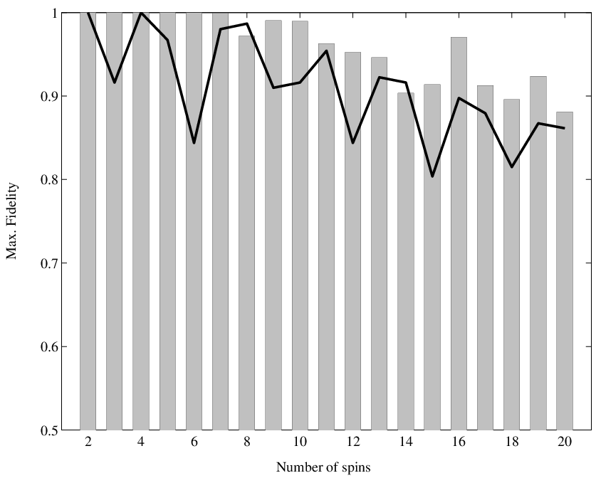
For asymptotically large $N$, using an expression for $f(t)$ in Ref. Christandl03 for the XY chain,

where $E_{m}=-2\omega\cos{\frac{m\pi}{N+1}}$. Let $J_{k}$ be the Bessel functions. The Jacobi-Anger expansion Arfken; mathca states that

Applying this to (40), taking $N$ to be large and $t_{0}$ to be of order $N$, and neglecting the terms with $k\gg N$ or $k\ll N$, we have,

Since $N+2+\xi(N+2)^{1/3}\approx N+\xi N^{1/3}$ for all $\xi$, and $J_{N}(N+\xi N^{1/3})\approx(2/N)^{1/3}A(-2^{1/3}\xi)$ abramowitz, where $A(\cdot)$ is the Airy function, applying $2\omega t_{0}=N+0.8089N^{1/3}$ gives a lower bound on the fidelity

This is twice the value of $f(t_{0})$ for a Heisenberg chain (3) for the same $t_{0}$ Bose03.

Although perfect state transfer is possible only for $N=2$ and $N=3$, fidelities very close to 1 are obtainable for sufficiently long evolution times. Such long evolution times can be shortened using a non-homogeneous magnetic field applied to individual spins. For example, for an $N=4$ XY chain, the maximum fidelity obtained is $0.99997$ at $t=53.4/\omega$, in the time interval of ($0,100/\omega$). However, if we apply a magnetic field of strength $B=0.625\omega$ on the two middle spins only, the fidelity is $0.99991$ at $t=6.25/\omega$, see Fig. 4.

References

- (1) N. Linden, H. Barjat, R. Carbajo, and R. Freeman, Chem. Phys. Lett. 305 28, (1999); D. W. Leung, I. L. Chuang, F. Yamaguchi, and Y. Yamamoto, Phys. Rev. A 61, 042310 (2000); J. Jones and E. Knill. J. of Mag. Res. 141, 322 (1999); J. L. Dodd, M. A. Nielsen, M. J. Bremner, R. T. Thew, Phys. Rev. A 65, 040301 (R) (2002); P. Wocjan, D. Janzing, Th. Beth, Quant. Inf. Comp. 2, 117 (2002); D. Leung, J. Mod. Opt. 49, 1199 (2002); M. Stollsteimer and G. Mahler, Phys. Rev. A 64, 052301 (2001); N. Khaneja, R. Brockett, and S. J. Glaser, Phys. Rev. A. 63, 032308 (2001); P. Wocjan, M. Roetteler, D. Janzing, and Th. Beth, Phys. Rev. A 65, 042309 (2002); M. A. Nielsen, M. J. Bremner, J. L. Dodd, A. M. Childs, C. M. Dawson, Phys. Rev. A 66, 022317 (2002).
- (2) D. W. Leung, I. L. Chuang, F. Yamaguchi, and Y. Yamamoto. Phys. Rev. A, 61 042310 (2000).
- (3) J. Jones and E. Knill. J. of Mag. Res., 141 322–5 (1999).
- (4) S. Bose, Phys. Rev. Lett 91, 207901 (2003).
- (5) V. Subrahmanyam, quan-ph/0307135.
- (6) M. Christandl, N. Datta, A. Ekert and A.J. Landahl, quan-ph/0309131.
- (7) N. Khaneja, S. J. Glaser and R. W. Brockett, Phys. Rev. A, , 032301 (2002).
- (8) T. S. Cubitt, F. Verstraete, W. Dr and J.I. Cirac, Phys. Rev. Lett. , 037902 (2003)
- (9) S. C. Benjamin and S. Bose, Phys. Rev. Lett. 90, 247901 (2003).
- (10) C. Bennett, A. Harrow, D. Leung, and J. Smolin, IEEE Trans. Inf. Theory, 580 (2002).
- (11) W. Dr, G. Vidal and J. I. Cirac, Phys. Rev. A , 062314 (2000).
- (12) A. Childs, E. Farhi, J. Goldstone, and S. Gutmann, Quant. Inf. Comp. , 181 (2002).
- (13) G. Arfken and H. Weber, Mathematical Methods for Physicists (Harcourt, San Diego, 2001).
- (14) Weisstein Mathematics, http://mathworld.wolfram.com
- (15) M. Abramowitz and I. A. Stegun, Handbook of Mathematical Functions (Dover, New York, 1972).