跳到论文正文
W Papers独立论文阅读器 arXiv:quant-ph/0312022 论文正文 计算阅读时间 · 0%
引用这篇论文根据当前论文元数据生成,正式投稿前建议核对。


License: Assumed arXiv.org perpetual non-exclusive license
arXiv:quant-ph/0312022v1 [quant-ph] 02 Dec 2003

Quantum Search Algorithm with more Reliable Behaviour using Partial Diffusion

Ahmed Younes         Jon Rowe Note: Birmingham, Edgbaston, B15 2TT, United Kingdom , axy@cs.bham.ac.uk Note: Birmingham, Edgbaston, B15 2TT, United Kingdom , jer@cs.bham.ac.uk Affiliation: School of Computer Science Affiliation: University of Birmingham    Julian Miller Note: York, Heslington, YO10 5DD, United Kingdom, jfm@ohm.york.ac.uk Affiliation: Department of Electronics Affiliation: University of York
Abstract

In this paper, we will use a quantum operator which performs the inversion about the mean operation only on a subspace of the system (Partial Diffusion Operator) to propose a quantum search algorithm runs in O⁡(N/M)O(\sqrt{N/M}) for searching unstructured list of size NN with MM matches such that, 1≤M≤N1\leq M\leq N. We will show that the performance of the algorithm is more reliable than known quantum search algorithms especially for multiple matches within the search space. A performance comparison with Grover’s algorithm will be provided.

1 Introduction

Quantum computers [6, 8, 12] are probabilistic devices, which promise to do some types of computation more powerfully than classical computers [3, 15]. Many quantum algorithms have been presented recently, for example, Shor [17] presented a quantum algorithm for factorising a composite integer into its prime factors in polynomial time. Grover [10] presented an algorithm for searching unstructured list of NN items with quadratic speed-up over algorithms run on classical computers.

Grover’s algorithm inspired many researchers, including this work, to try to analyze and/or generalize his algorithm [1, 4, 5, 9, 11, 18]. Grover’s algorithm perfomance is near to optimum for a single match within the search space, although the number of iterations required by the algorithm increases; i.e. the problem becomes harder, as the number of matches exceeds half the number of items in the search space [13] which is undesired behaviour for a search algorithm since the problem is expected to be easier for multiple matches.

In this paper, using a partial diffusion operation, we will show a quantum algorithm, which can find a match among multiple matches within the search space after one iteration with probability at least 90% if the number of matches is more than one-third of the search space. For fewer matches the algorithm runs in quadratic speed up similar to Grover’s algorithm with more reliable behaviour, as we will see.

The plan of the paper is as follows: Section 2 gives a short introduction to quantum computers. Section 3 introduces the search problem and Grover’s algorithm performance. Section 4 and 5 introduce the proposed algorithm with analysis on its performance and behaviour. And we will end up with a conclusion in section 6.

2 Quantum Computers

2.1 Quantum Bits

In classical computers, a bit is considered as the basic unit for information processing; a bit can carry one value at a time (either 0 or 1). In quantum computers, the analogue of the bit is the quantum bit (qubit [16]), which has two possible states encoded as |0⟩\left|0\right\rangle and |1⟩\left|1\right\rangle; where the notation |⟩\left|\,\,\,\right\rangle is called Dirac Notation and is considered as the standard notation of states in quantum mechanics [7]. For quantum computing purposes, the states |0⟩\left|0\right\rangle and |1⟩\left|1\right\rangle can be considered as the classical bit values 0 and 1 respectively. An important difference between a classical bit and a qubit is that the qubit can exist in a linear superposition of both states (|0⟩\left|0\right\rangle and |1⟩)\left|1\right\rangle) at the same time and this gives the hope that quantum computers can do computation simultaneously (Quantum Parallelism). If we consider a quantum register with nn qubits all in superposition, then any operation applied on this register will be applied on the 2n2^{n} states representing the superposition simultaneously.

2.2 Quantum Measurements

To read information from a quantum register (quantum system), we must apply a measurement on that register which will result in a projection of the states of the system to a subspace of the state space compatible with the values being measured. For example, consider a two-qubit system |ϕ⟩\left|\phi\right\rangle defined as follows:

|ϕ⟩=α|00⟩+β|01⟩+γ|10⟩+δ|11⟩,\left|\phi\right\rangle=\alpha\left|{00}\right\rangle+\beta\left|{01}\right\rangle+\gamma\left|{10}\right\rangle+\delta\left|{11}\right\rangle, (1)

where α\alpha, β\beta, γ\gamma, and δ\delta are complex numbers called the amplitudes of the system and satisfy |α|2+|β|2+|γ|2+|δ|2=1\left|\alpha\right|^{2}+\left|\beta\right|^{2}+\left|\gamma\right|^{2}+\left|\delta\right|^{2}=1. The probability that the first qubit of |ϕ⟩\left|\phi\right\rangle to be |0⟩\left|0\right\rangle is equal to (|α|2+|β|2)\left({\left|\alpha\right|^{2}+\left|\beta\right|^{2}}\right). If for some reasons we need to have the value |0⟩\left|0\right\rangle in the first qubit after any measurement, we must try some how to increase its probability before applying the measurement. Note that, the new state after applying measurement must be re-normalized so the total probability is still 1.

2.3 Quantum Gates

In general, quantum algorithms can be understood as follows: Apply a series of transformations (gates) then apply the measurement to get the desired result with high probability. According to the laws of quantum mechanics and to keep the reversibility condition required in quantum computation, the evolution of the state of the quantum system |ψ⟩\left|\psi\right\rangle of size nn by time tt is described by a matrix UU of dimension 2n×2n2^{n}\times 2^{n} [13]:

|ψ′⟩=U|ψ⟩,\left|{\psi^{\prime}}\right\rangle=U\left|\psi\right\rangle, (2)

where UU satisfies the unitary condition: U†​U=IU^{{\dagger}}U=I, where U†U^{{\dagger}} denotes the complex conjugate transpose of UU and II is the identity matrix. For example, the XX gate (N​O​TNOT gate) is a single qubit gate (single input/output) similar in its effect to the classical N​O​TNOT gate. It inverts the state |0⟩\left|0\right\rangle to the state |1⟩\left|1\right\rangle and visa versa. It’s 2×22\times 2 unitary matrix takes this form,

X=[0110],X=\left[{{\begin{array}[]{*{20}c}0\hfill&1\hfill\\ 1\hfill&0\hfill\\ \end{array}}}\right], (3)

and its circuit takes the form shown in Fig.(1). Notice that, from now on we assume that a horizontal line used in any quantum circuit represents a qubit and the flow of the circuit logic is from left to right. For circuits with multiple qubits, qubits will be arranged according to the notation used in the figure.

Figure 1: N​O​TNOT gate quantum circuit.

Another important example is the Hadamard gate (HH gate) which has no classical equivalent; it produces a completely random output with equal probabilities of the output to be |0⟩\left|0\right\rangle or |1⟩\left|1\right\rangle on any measurements. It’s 2×22\times 2 unitary matrix takes this form,

H=12​[1    11−1],H=\frac{1}{\sqrt{2}}\left[{{\begin{array}[]{*{20}c}1\hfill&\,\,\,\,1\hfill\\ 1\hfill&{-1}\hfill\\ \end{array}}}\right], (4)

and its circuit takes the form shown in Fig.(2).

Figure 2: Hadamard gate quantum circuit, where xx is any Boolean variable.

Controlled operations are considered as the heart of quantum computing [2], Controlled-UU gate is the general case for any controlled gate with one or more control qubit(s) as shown in Fig.(3.a). It works as follows: If any of the control qubits |ci⟩\left|{c_{i}}\right\rangle’s (OPEN1≤i≤n−1)1\leq i\leq n-1) is set to 0, then the quantum gate UU will not be applied on target qubit |t⟩\left|t\right\rangle; i.e. UU is applied on |t⟩\left|t\right\rangle if and only if all |ci⟩\left|{c_{i}}\right\rangle’s are set to 1. The states of the qubits after applying the gate will be transformed according to the following rule:

|ci⟩→|ci⟩;1≤i≤n−1|t⟩→|tC​U⟩=Uc1​c2​…​cn−1|t⟩\begin{array}[]{l}\left|{c_{i}}\right\rangle\to\left|{c_{i}}\right\rangle;1\leq i\leq n-1\\ \left|t\right\rangle\to\left|t_{CU}\right\rangle=U^{c_{1}c_{2}...c_{n-1}}\left|t\right\rangle\\ \end{array} (5)

where c1​c2​…​cn−1c_{1}c_{2}...c_{n-1} in the exponent of UU means the A​N​DAND-ing of the qubits c1,c2,…,cn−1c_{1},\,c_{2},...,c_{n-1}.

Figure 3: Controlled gates where the back circle ∙\bullet indicates the control qubits, and the symbol ⊕\oplus in part (b.) indicates the target qubit.

If UU in the general Controlled-UU gate is replaced with the XX gate mentioned above, the resulting gate is called Controlled-N​O​TNOT gate (shown in Fig.(3.b)). It works as follows: It inverts the target qubit if and only if all the control qubits are set to 1. Thus the qubits of the system will be transformed according to the following rule:

|ci⟩→|ci⟩;1≤i≤n−1|t⟩→|tC​N⟩=|t⊕c1c2…cn−1⟩\begin{array}[]{l}\left|{c_{i}}\right\rangle\to\left|{c_{i}}\right\rangle;1\leq i\leq n-1\\ \left|{t}\right\rangle\to\left|t_{CN}\right\rangle=\left|{t\oplus c_{1}c_{2}...c_{n-1}}\right\rangle\\ \end{array} (6)

where c1​c2​…​cn−1c_{1}c_{2}\ldots c_{n-1} is the A​N​DAND-ing of the qubits c1,c2,…,cn−1c_{1},c_{2},\ldots,c_{n-1} and ⊕\oplus is the classical XOR operation.

3 Search Problem

Consider a list LL of NN items; L={0,1,…,N−1}L=\{0,1,...,N-1\}, and consider a function ff which maps the items in LL to either 0 or 1 according to some properties these items shall satisfy; i.e. f:L→{0,1}f:L\to\{0,1\}. The problem is to find any i∈Li\in L such that f⁡(i)=1f(i)=1 assuming that such ii must exist in the list. It was shown classically that we need approximately N​/​2{N\mathord{\left/{\vphantom{N2}}\right.\kern-1.2pt}2} tests to get a result with probability at least one-half. Let MM denotes the number of matches within the search space such that 1≤M≤N1\leq M\leq N and for simplicity and without loss of generality we can assume that N=2nN=2^{n}. Grover’s algorithm was shown to solve this problem [4] in O⁡(N/M)O\left({\sqrt{N/M}}\right). In [13], it was shown that the number of iterations will increase for M>N/2M>N/2 which is undesired behaviour for a search algorithm. To over come this problem it was proposed in [13] that the search space can be doubled so the number of matches always less than half the search space and iterate the algorithm π/4​2​N/M\pi/4\sqrt{2N/M} times so the algorithm still runs in O⁡(N/M)O\left({\sqrt{N/M}}\right). But using this approach will double the cost of space/time requirement. In the following section we will present an algorithm that can find a solution for M>N/2M>N/2 with probability at least 92.6%92.6\% after applying the algorithm once.

4 The Algorithm

4.1 Iterating the algorithm once

Figure 4: Quantum circuit for the proposed algorithm.

For a list of size N=2nN=2^{n}, the steps of the algorithm can be understood as follows as shown in Fig.(4):

  • 1-

    Register Preparation. Prepare a quantum register of n+1n+1 qubits all in state |0⟩\left|0\right\rangle, where the extra qubit is used as a workspace for evaluating the oracle UfU_{f}:

    |W0⟩=|0⟩⊗n⊗|0⟩.\left|{W_{0}}\right\rangle=\left|0\right\rangle^{\otimes n}\otimes\left|0\right\rangle. (7)
  • 2-

    Register Initialization. Apply Hadamard gate on each of the first nn qubits in parallel, so they contain the 2n2^{n} states, where ii is the integer representation of items in the list:

    |W1⟩=(H⊗n⊗I)|W0⟩=(1N∑i=0N−1|i⟩)⊗|0⟩.\left|{W_{1}}\right\rangle=\left({H^{\otimes n}\otimes I}\right)\left|{W_{0}}\right\rangle=\left({\frac{1}{\sqrt{N}}\sum\limits_{i=0}^{N-1}{\left|i\right\rangle}}\right)\otimes\left|0\right\rangle. (8)
  • 3-

    Applying Oracle. Apply the oracle UfU_{f} to map the items in the list to either 0 or 1 simultaneously and stores the result in the extra workspace qubit:

    |W2⟩=1N∑i=0N−1(|i⟩⊗|0⊕f(i)⟩)=1N∑i=0N−1(|i⟩⊗|f(i)⟩).\left|{W_{2}}\right\rangle=\frac{1}{\sqrt{N}}\sum\limits_{i=0}^{N-1}{\left({\left|i\right\rangle\otimes\left|{0\oplus f(i)}\right\rangle}\right)}=\frac{1}{\sqrt{N}}\sum\limits_{i=0}^{N-1}{\left({\left|i\right\rangle\otimes\left|{f(i)}\right\rangle}\right)}. (9)
  • 4-

    Partial Diffusion. In this step, we will define a new operator: Partial Diffusion Operator (Y)(Y) which works similar to the well known Diffusion Operator used in Grover’s algorithm [10] except that it performs the inversion about the mean operation only on a subspace of the system as follows: The diagonal representation of the partial diffusion operator YY when applied on n+1n+1 qubits system can take this form:

    Y=H⊗n⊗I(2|0⟩⟨0|−I)H⊗n⊗I,Y=H^{\otimes n}\otimes I\left({2\left|0\right\rangle\left\langle 0\right|-I}\right)H^{\otimes n}\otimes I, (10)

    where the vector |0⟩\left|0\right\rangle used in Eqn.(10) is a vector of lenght P=2​N=2n+1P=2N=2^{n+1}. Applying YY on a general system ∑k=0P−1δk|k⟩\sum\nolimits_{k=0}^{P-1}{\delta_{k}\left|k\right\rangle}; where, |δk|2=1\left|{\delta_{k}}\right|^{2}=1, can be understood as follows: Without loosing of generality, the general system can be re-written as,

    ∑k=0P−1δk|k⟩=∑j=0N−1αj(|j⟩⊗|0⟩)+∑j=0N−1βj(|j⟩⊗|1⟩),\sum\limits_{k=0}^{P-1}{\delta_{k}\left|k\right\rangle}=\sum\limits_{j=0}^{N-1}{\alpha_{j}\left({\left|j\right\rangle\otimes\left|0\right\rangle}\right)}+\sum\limits_{j=0}^{N-1}{\beta_{j}\left({\left|j\right\rangle\otimes\left|1\right\rangle}\right)}, (11)

    where {αj=δk\alpha_{j}=\delta_{k} : kk even} and {βj=δk\beta_{j}=\delta_{k} : kk odd}, then applying YY on the system gives,

    Y(∑k=0P−1δk|k⟩)=(H⊗n⊗I(2|0⟩⟨0|−I)H⊗n⊗I)∑k=0P−1δk|k⟩=2(H⊗n⊗I|0⟩⟨0|H⊗n⊗I)∑k=0P−1δk|k⟩−∑k=0P−1δk|k⟩=∑j=0N−1(2⟨α⟩−αj)(|j⟩⊗|0⟩)−∑j=0N−1βj(|j⟩⊗|1⟩),\begin{array}[]{l}Y\left({\sum\limits_{k=0}^{P-1}{\delta_{k}\left|k\right\rangle}}\right)=\left({H^{\otimes n}\otimes I\left({2\left|0\right\rangle\left\langle 0\right|-I}\right)H^{\otimes n}\otimes I}\right)\sum\limits_{k=0}^{P-1}{\delta_{k}\left|k\right\rangle}\\ \,\,\,\,\,\,\,\,\,\,\,\,\,\,\,\,\,\,\,\,\,\,\,\,\,\,\,\,\,\,\,\,\,\,\,\,\,\,\,=2\left({H^{\otimes n}\otimes I\left|0\right\rangle\left\langle 0\right|H^{\otimes n}\otimes I}\right)\sum\limits_{k=0}^{P-1}{\delta_{k}\left|k\right\rangle}-\sum\limits_{k=0}^{P-1}{\delta_{k}\left|k\right\rangle}\\ \,\,\,\,\,\,\,\,\,\,\,\,\,\,\,\,\,\,\,\,\,\,\,\,\,\,\,\,\,\,\,\,\,\,\,\,\,\,\,=\sum\limits_{j=0}^{N-1}{\left({2\left\langle\alpha\right\rangle-\alpha_{j}}\right)\left({\left|j\right\rangle\otimes\left|0\right\rangle}\right)}-\sum\limits_{j=0}^{N-1}{\beta_{j}\left({\left|j\right\rangle\otimes\left|1\right\rangle}\right)},\\ \end{array} (12)

    where ⟨α⟩=1N​∑j=0N−1αj\left\langle\alpha\right\rangle=\frac{1}{N}\sum\nolimits_{j=0}^{N-1}{\alpha_{j}} is the mean of the amplitudes of the subspace ∑j=0N−1αj(|j⟩⊗|0⟩)\sum\nolimits_{j=0}^{N-1}{\alpha_{j}\left({\left|j\right\rangle\otimes\left|0\right\rangle}\right)}; i.e. applying the operator YY will perform the inversion about the mean only on the subspace; ∑j=0N−1αj(|j⟩⊗|0⟩)\sum\nolimits_{j=0}^{N-1}{\alpha_{j}\left({\left|j\right\rangle\otimes\left|0\right\rangle}\right)} and will only change the sign of the amplitudes for the rest of the system; ∑j=0N−1βj(|j⟩⊗|1⟩)\sum\nolimits_{j=0}^{N-1}{\beta_{j}\left({\left|j\right\rangle\otimes\left|1\right\rangle}\right)}, a circuit implementation using elementary gates [2] is shown in Fig.(5).

    Figure 5: Quantum circuit representing the Partial Diffusion Operator YY over n+1n+1 qubits.

    The main idea of using the partial diffusion operator in searching is to apply the inversion about the mean operation only on the subspace of the system which includes all the states which represent the non-matches and half the number of the states which represent the matches while the other half will have the sign of their amplitudes inverted to the negative sign preparing them to be involved in the partial diffusion operation in the next iteration so the amplitudes of the matching states get amplified partially each iteration. The benefit of this is to keep half the number of the states which represent the matches as a stock each iteration to resist the de-amplification behaviour of the diffusion operation when reaching the turning points as we will see when examining the performance of the algorithm.

    Let MM be the number of matches, which makes the oracle UfU_{f} evaluate to TRUE (solutions); such that 1≤M≤N1\leq M\leq N; assume that ∑i′\sum\nolimits_{i}{{{}^{\prime}}} indicates a sum over all ii which are desired matches (MM states), and ∑i′′\sum\nolimits_{i}{{{}^{\prime\prime}}} indicates a sum over all ii which are undesired items in the list. So, the system |W2⟩\left|{W_{2}}\right\rangle shown in Eqn.(9) can be written as follows:

    |W2⟩=1N∑i=0N−1(|i⟩′′⊗|0⟩)+1N∑i=0N−1(|i⟩′⊗|1⟩).\left|{W_{2}}\right\rangle=\frac{1}{{\sqrt{N}}}\sum\limits_{i=0}^{N-1}{{}^{\prime\prime}\left({\left|i\right\rangle\otimes\left|0\right\rangle}\right)}+\frac{1}{{\sqrt{N}}}\sum\limits_{i=0}^{N-1}{{}^{\prime}\left({\left|i\right\rangle\otimes\left|1\right\rangle}\right)}. (13)

    Applying YY on |W2⟩\left|{W_{2}}\right\rangle will result in a new system described as follows:

    |W3⟩=a1∑i=0N−1(|i⟩′′⊗|0⟩)+b1∑i=0N−1(|i⟩′⊗|0⟩)+c1∑i=0N−1(|i⟩′⊗|1⟩),\left|{W_{3}}\right\rangle=a_{1}\sum\limits_{i=0}^{N-1}{{}^{\prime\prime}\left({\left|i\right\rangle\otimes\left|0\right\rangle}\right)}+b_{1}\sum\limits_{i=0}^{N-1}{{}^{\prime}\left({\left|i\right\rangle\otimes\left|0\right\rangle}\right)}+c_{1}\sum\limits_{i=0}^{N-1}{{}^{\prime}\left({\left|i\right\rangle\otimes\left|1\right\rangle}\right)}, (14)

    where the mean used in the definition of partial diffusion operator is,

    ⟨α1⟩=(N−MN​N),\left\langle{\alpha_{1}}\right\rangle=\left({\frac{{N-M}}{{N\sqrt{N}}}}\right), (15)

    and a1a_{1}, b1b_{1} and c1c_{1} used in Eqn.(14) are calculates as follows:

    a1=2​⟨α1⟩−1N;b1=2​⟨α1⟩;c1=−1N.a_{1}=2\left\langle{\alpha_{1}}\right\rangle-\frac{1}{{\sqrt{N}}};\,\,\,\,\,\ b_{1}=2\left\langle{\alpha_{1}}\right\rangle;\,\,\,\,\,\ c_{1}=\frac{{-1}}{{\sqrt{N}}}. (16)

    Such that,

    (N−M)​a12+M​b12+M​c12=1.\left({N-M}\right)a_{1}^{2}+Mb_{1}^{2}+Mc_{1}^{2}=1. (17)

    Notice that, the states with amplitude b1b_{1} was with amplitude zero before applying YY.

  • 5-

    Measurement. If we measure the first nn qubits after the first iteration (q=1q=1), we will get the desired solution with probability given as follows:

    • i-

      Probability Ps(1)P_{s}^{(1)} to find a match out of the MM possible matches; taking into account that a solution |i⟩\left|i\right\rangle occurs twice as: (|i⟩⊗|0⟩)\left({\left|i\right\rangle\otimes\left|0\right\rangle}\right) with amplitude b1b_{1} and (|i⟩⊗|1⟩)\left({\left|i\right\rangle\otimes\left|1\right\rangle}\right) with amplitude c1c_{1} as shown in Eqn.(14), can be calculated as follows:

      Ps(1)=M⁡(b12+c12)=M⁡((2​(N−M)N​N)2+(−1N)2)=5​(MN)−8​(MN)2+4​(MN)3.\begin{array}[]{l}P_{s}^{(1)}=M\left({b_{1}^{2}+c_{1}^{2}}\right)\\ \,\,\,\,\,\,\,=M\left({\left({\frac{{2\left({N-M}\right)}}{{N\sqrt{N}}}}\right)^{2}+\left({\frac{{-1}}{{\sqrt{N}}}}\right)^{2}}\right)\\ \,\,\,\,\,\,\,=5\left({\frac{M}{N}}\right)-8\left({\frac{M}{N}}\right)^{2}+4\left({\frac{M}{N}}\right)^{3}.\\ \end{array} (18)
    • ii-

      Probability Pn​s(1)P_{ns}^{(1)} to find undesired result out of the states can be calculated as follows:

      Pn​s(1)=(N−M)​a12.P_{ns}^{(1)}=(N-M)a_{1}^{2}. (19)

      Notice that, using Eqn.(17),

      Ps(1)+Pn​s(1)=1.P_{s}^{(1)}+P_{ns}^{(1)}=1. (20)

4.1.1 Performance after Iterating the Algorithm Once

nn, where N=2nN=2^{n} Max. prob. Min. prob. Avg. prob.
2 1.0 0.8125 0.875
3 1.0 0.507812 0.937500
4 1.0 0.282227 0.968750
5 1.0 0.148560 0.984375
6 1.0 0.076187 0.992187
Table 1: First iteration performance with different size search space.

Considering Eqn.(14) and Eqn.(18) we can see that the probability to find a solution varies according to the number of matches MM in the superposition.

From Table.1, we can see that the maximum probability is always 1.0, and the minimum probability (worst case) decreases as the size of the list increases, which is expected for small MM because the number of states will increase and the probability shall distribute over more states while the average probability increases as the size of the list increases. It implies that the average performance of the first iteration of algorithm to find a solution increases as the size of the list increases.

To verify these results, taking into account that the oracle UfU_{f} is taken as a black box, we can define the average probability of success of the first iteration of algorithm; a​v​e​r​a​g​e​(Ps(1))average(P_{s}^{(1)}), as follows:

a​v​e​r​a​g​e​(Ps(1))=12N​∑M=1NCMN​Ps(1)=12N​∑M=1NN!M!​(N−M)!.M⁡(b12+c12)=12N+1​N3​∑M=1NN!(M−1)!​(N−M)!​(10​N2−16​M​N+8​M2)=1−12​N.\begin{array}[]{l}average(P_{s}^{(1)})=\frac{1}{{2^{N}}}\sum\limits_{M=1}^{N}{{}^{N}C_{M}P_{s}^{(1)}}\\ \,\,\,\,\,\,\,\,\,\,\,\,\,\,\,\,\,\,\,\,\,\,\,\,\,\,=\frac{1}{{2^{N}}}\sum\limits_{M=1}^{N}{\frac{{N!}}{{M!(N-M)!}}.M\left({b_{1}^{2}+c_{1}^{2}}\right)}\\ \,\,\,\,\,\,\,\,\,\,\,\,\,\,\,\,\,\,\,\,\,\,\,\,\,\,=\frac{1}{{2^{N+1}N^{3}}}\sum\limits_{M=1}^{N}{\frac{{N!}}{{(M-1)!(N-M)!}}\left({10N^{2}-16MN+8M^{2}}\right)}\\ \,\,\,\,\,\,\,\,\,\,\,\,\,\,\,\,\,\,\,\,\,\,\,\,\,\,=1-\frac{1}{{2N}}.\\ \end{array} (21)

where CMN=N!M!​(N−M)!{}^{N}C_{M}=\frac{{N!}}{{M!(N-M)!}} is the number of possible cases for MM matches.

We can see that as the size of the list increases (N→∞)(N\to\infty), a​v​e​r​a​g​e​(Ps(1))average(P_{s}^{(1)}) shown in Eqn.(21) tends to 11.

Classically, we can try to find a random guess of the item, which represents the solution (one trial guess), we may succeed to find a solution with probability Ps(c​l​a​s​s​i​c​a​l)=M/NP^{(classical)}_{s}=M/N. The average probability of success can be calculated as follows:

a​v​e​r​a​g​e​(Ps(c​l​a​s​s​i​c​a​l))=12N​∑M=1NCMN​Ps(c​l​a​s​s​i​c​a​l)=12N​∑M=1NN.MM!​(N−M)!​N=12.\begin{array}[]{l}average(P_{s}^{(classical)})=\frac{1}{{2^{N}}}\sum\limits_{M=1}^{N}{{}^{N}C_{M}P_{s}^{(classical)}}\\ \,\,\,\,\,\,\,\,\,\,\,\,\,\,\,\,\,\,\,\,\,\,\,\,\,\,\,\,\,\,\,\,\,\,\,\,\,\,\,\,\,\,\,\,\,\,\,\,\,\,\,\,\,\,\,=\frac{1}{{2^{N}}}\sum\limits_{M=1}^{N}{\frac{{N.M}}{{M!(N-M)!N}}}\\ \,\,\,\,\,\,\,\,\,\,\,\,\,\,\,\,\,\,\,\,\,\,\,\,\,\,\,\,\,\,\,\,\,\,\,\,\,\,\,\,\,\,\,\,\,\,\,\,\,\,\,\,\,\,\,=\frac{1}{2}.\\ \end{array} (22)

It means that we have an average probability one-half to find or not to find a solution by a single random guess even with the increase in size of the list.

Similarly, Grover’s algorithm has an average probabilty one-half after arbitrary number of iterations as we will see. It was shown in [4] that the probability of success of Grover’s algorithm after qGq_{G} iterations is given by:

Ps(qG)=sin2⁡((2​qG+1)​θ),where, ​ 0<θ≤π2​ and ​sin2⁡(θ)=MN.P_{s}^{(q_{G})}=\sin^{2}((2q_{G}+1)\theta),\,\,\,\mbox{where, }\,0<\theta\leq\frac{\pi}{2}\mbox{ and }\sin^{2}(\theta)=\frac{M}{N}.\\ (23)

The average probability of success of Grover’s algorithm after arbitrary number of iterations is as follows (Appendix A in [18]):

a​v​e​r​a​g​e​(Ps(qG))=12N​∑M=1NCMN​sin2⁡((2​qG+1)​θ)=12.average(P_{s}^{(q_{G})})=\frac{1}{{2^{N}}}\sum\limits_{M=1}^{N}{{}^{N}C_{M}\sin^{2}((2q_{G}+1)\theta)}=\frac{1}{2}.\\ (24)

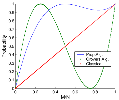
Comparing the performance of the first iteration of the proposed algorithm, first iteration of Grover’s algorithm and the classical guess technique, Fig.(6) shows the probability of success of the three algorithms just mentioned as a function of the ratio (M/N)(M/N).

Refer to caption

Figure 6: A plot of the probability of success of the first the iteration of proposed algorithm Ps(1)P_{s}^{(1)}, first iteration of Grover’s algorithm Ps(1G)P_{s}^{(1_{G})} and the classical guess Ps(c​l​a​s​s​i​c​a​l)P_{s}^{(classical)} as a function of the ratio (M/N)(M/N).

We can see from Fig.(6) that the probability of success of the first iteration is always above that of the classical guess technique. Grover’s algorithm solves the case where M=N/4M=N/4 with certainity and the proposed algorithm solves the case where M=N/2M=N/2 with certainity. The probability of success of Grover’s algorithm will start to go below one-half for M>N/2M>N/2 while the probability of success of the proposed algorithm will stay more reliable with propabilty at least 92.6%92.6\%.

4.2 Iterating the Algorithm

If we consider iterating the algorithm, the iterating block will be applying the oracle UfU_{f} and the operator YY on the system in sequence as shown in Fig.(4). To understand the effect of each iteration on the system, we will trace the state of the system during the first few iterations. Consider the system after first iteration shown in Eqn.(14), second iteration will modify the system as follows:

Apply the oracle UfU_{f} will swap the amplitudes of the states which represent only the matches, i.e. states with amplitudes b1b_{1} will be with amplitudes c1c_{1} and states with amplitudes c1c_{1} will be with amplitudes b1b_{1} so the system can be described as,

|W4⟩=a1∑i=0N−1(|i⟩′′⊗|0⟩)+c1∑i=0N−1(|i⟩′⊗|0⟩)+b1∑i=0N−1(|i⟩′⊗|1⟩).\left|{W_{4}}\right\rangle=a_{1}\sum\limits_{i=0}^{N-1}{{}^{\prime\prime}\left({\left|i\right\rangle\otimes\left|0\right\rangle}\right)}+c_{1}\sum\limits_{i=0}^{N-1}{{}^{\prime}\left({\left|i\right\rangle\otimes\left|0\right\rangle}\right)}+b_{1}\sum\limits_{i=0}^{N-1}{{}^{\prime}\left({\left|i\right\rangle\otimes\left|1\right\rangle}\right)}. (25)

Applying the operator YY will change the system as follows,

|W5⟩=a2∑i=0N−1(|i⟩′′⊗|0⟩)+b2∑i=0N−1(|i⟩′⊗|0⟩)+c2∑i=0N−1(|i⟩′⊗|1⟩),\left|{W_{5}}\right\rangle=a_{2}\sum\limits_{i=0}^{N-1}{{}^{\prime\prime}\left({\left|i\right\rangle\otimes\left|0\right\rangle}\right)}+b_{2}\sum\limits_{i=0}^{N-1}{{}^{\prime}\left({\left|i\right\rangle\otimes\left|0\right\rangle}\right)}+c_{2}\sum\limits_{i=0}^{N-1}{{}^{\prime}\left({\left|i\right\rangle\otimes\left|1\right\rangle}\right)}, (26)

where the mean used in the definition of partial diffusion operator is,

⟨α2⟩=1N​((N−M)​a1+M​c1),\left\langle{\alpha_{2}}\right\rangle=\frac{1}{N}\left({\left({N-M}\right)a_{1}+Mc_{1}}\right), (27)

and a2a_{2}, b2b_{2} and c2c_{2} used in Eqn.(26) are calculated as follows:

a2=2​⟨α2⟩−a1;b2=2​⟨α2⟩−c1;c2=−b1,a_{2}=2\left\langle{\alpha_{2}}\right\rangle-a_{1};\,\,\,\,\,\,\,\,b_{2}=2\left\langle{\alpha_{2}}\right\rangle-c_{1};\,\,\,\,\,\,c_{2}=-b_{1}, (28)

and the probabilities of the system are,

Ps(2)=M⁡(b22+c22)=M⁡(b22+b12).Pn​s(2)=M⁡(a22)=M​(b2+c2)2=M​(b2−b1)2.\begin{array}[]{l}P_{s}^{(2)}=M\left({b_{2}^{2}+c_{2}^{2}}\right)=M\left({b_{2}^{2}+b_{1}^{2}}\right).\\ P_{ns}^{(2)}=M\left({a_{2}^{2}}\right)=M\left({b_{2}+c_{2}}\right)^{2}=M\left({b_{2}-b_{1}}\right)^{2}.\\ \end{array} (29)

In the same fashion, third iteration will give the following system,

Uf|W5⟩=|W6⟩=a2∑i=0N−1(|i⟩′′⊗|0⟩)+c2∑i=0N−1(|i⟩′⊗|0⟩)+b2∑i=0N−1(|i⟩′⊗|1⟩)U_{f}\left|{W_{5}}\right\rangle=\left|{W_{6}}\right\rangle=a_{2}\sum\limits_{i=0}^{N-1}{{}^{\prime\prime}\left({\left|i\right\rangle\otimes\left|0\right\rangle}\right)}+c_{2}\sum\limits_{i=0}^{N-1}{{}^{\prime}\left({\left|i\right\rangle\otimes\left|0\right\rangle}\right)}+b_{2}\sum\limits_{i=0}^{N-1}{{}^{\prime}\left({\left|i\right\rangle\otimes\left|1\right\rangle}\right)} (30)
Y|W6⟩=|W7⟩=a3∑i=0N−1(|i⟩′′⊗|0⟩)+b3∑i=0N−1(|i⟩′⊗|0⟩)+c3∑i=0N−1(|i⟩′⊗|1⟩),Y\left|{W_{6}}\right\rangle=\left|{W_{7}}\right\rangle=a_{3}\sum\limits_{i=0}^{N-1}{{}^{\prime\prime}\left({\left|i\right\rangle\otimes\left|0\right\rangle}\right)}+b_{3}\sum\limits_{i=0}^{N-1}{{}^{\prime}\left({\left|i\right\rangle\otimes\left|0\right\rangle}\right)}+c_{3}\sum\limits_{i=0}^{N-1}{{}^{\prime}\left({\left|i\right\rangle\otimes\left|1\right\rangle}\right)}, (31)

where the mean used in the definition of partial diffusion operator is,

⟨α3⟩=1N​((N−M)​a2+M​c2),\left\langle{\alpha_{3}}\right\rangle=\frac{1}{N}\left({\left({N-M}\right)a_{2}+Mc_{2}}\right), (32)

and a3a_{3}, b3b_{3} and c3c_{3} used in Eqn.(31) are calculated as follows:

a3=2​⟨α3⟩−a2;b3=2​⟨α3⟩−c2;c3=−b2,a_{3}=2\left\langle{\alpha_{3}}\right\rangle-a_{2};\,\,\,\,\,\,\,\,b_{3}=2\left\langle{\alpha_{3}}\right\rangle-c_{2};\,\,\,\,\,\,c_{3}=-b_{2}, (33)

and the probabilities of the system are,

Ps(3)=M⁡(b32+c32)=M⁡(b32+b22).Pn​s(3)=M⁡(a32)=M​(b3+c3)2=M​(b3−b2)2.\begin{array}[]{l}P_{s}^{(3)}=M\left({b_{3}^{2}+c_{3}^{2}}\right)=M\left({b_{3}^{2}+b_{2}^{2}}\right).\\ P_{ns}^{(3)}=M\left({a_{3}^{2}}\right)=M\left({b_{3}+c_{3}}\right)^{2}=M\left({b_{3}-b_{2}}\right)^{2}.\\ \end{array} (34)

In general, the system after q≥2q\geq 2 iterations can be described using the following recurrence relations,

|W(q)⟩=aq∑i=0N−1(|i⟩′′⊗|0⟩)+bq∑i=0N−1(|i⟩′⊗|0⟩)+cq∑i=0N−1(|i⟩′⊗|1⟩),\left|{W^{(q)}}\right\rangle=a_{q}\sum\limits_{i=0}^{N-1}{{}^{\prime\prime}\left({\left|i\right\rangle\otimes\left|0\right\rangle}\right)}+b_{q}\sum\limits_{i=0}^{N-1}{{}^{\prime}\left({\left|i\right\rangle\otimes\left|0\right\rangle}\right)}+c_{q}\sum\limits_{i=0}^{N-1}{{}^{\prime}\left({\left|i\right\rangle\otimes\left|1\right\rangle}\right)}, (35)

where the mean to be used in the definition of the partial diffusion operator is as follows: For simplicity, let y=1−MNy=1-\frac{M}{N} and s=1Ns=\frac{1}{\sqrt{N}}, then

⟨αq⟩=(y​aq−1+(1−y)​cq−1),\left\langle{\alpha_{q}}\right\rangle=\left({ya_{q-1}+(1-y)c_{q-1}}\right), (36)

and aqa_{q}, bqb_{q} and cqc_{q} used in Eqn.(35) are calculated as follows:

aq=2​⟨αq⟩−aq−1;a0=s,a1=s⁡(2​y−1),a_{q}=2\left\langle{\alpha_{q}}\right\rangle-a_{q-1};\,\,\,\,a_{0}=s,\,\,\,\,a_{1}=s\left({2y-1}\right), (37)
bq=2​⟨αq⟩−cq−1;b0=s,b1=2​s​y,b_{q}=2\left\langle{\alpha_{q}}\right\rangle-c_{q-1};\,\,\,\,\,b_{0}=s,\,\,\,\,b_{1}=2sy, (38)
cq=−bq−1;c0=0,c1=−s,c_{q}=-b_{q-1};\,\,\,\,\,\,\,\,\,\,\,\,\,\,\,\,\,\,c_{0}=0,\,\,\,\,c_{1}=-s, (39)

and the probabilities of the system are,

Ps(q)=M⁡(bq2+cq2)=M⁡(bq2+bq−12).P_{s}^{(q)}=M\left({b_{q}^{2}+c_{q}^{2}}\right)=M\left({b_{q}^{2}+b_{q-1}^{2}}\right). (40)
Pn​s(q)=M⁡(aq2)=M​(bq+cq)2=M​(bq−bq−1)2.P_{ns}^{(q)}=M\left({a_{q}^{2}}\right)=M\left({b_{q}+c_{q}}\right)^{2}=M\left({b_{q}-b_{q-1}}\right)^{2}. (41)

For q≥2q\geq 2, Eqn.(37), Eqn.(38) and Eqn.(39) could be re-written as follows:

aq=2​y​aq−1−aq−2;a0=s;a1=s⁡(2​y−1),a_{q}=2ya_{q-1}-a_{q-2};\,\,\,\,\,a_{0}=s;\,\,\,\,\,a_{1}=s(2y-1), (42)
bq=2​y​bq−1−bq−2;b0=s;b1=2​s​y,b_{q}=2yb_{q-1}-b_{q-2};\,\,\,\,\,\,b_{0}=s;\,\,\,\,\,b_{1}=2sy, (43)
cq=−bq−1;c0=0;c1=−s,c_{q}=-b_{q-1};\,\,\,\,\,\,\,\,\,\,\,\,\,\,\,\,\,\,\,\,\,c_{0}=0;\,\,\,\,c_{1}=-s, (44)

Solving the above recurrence relations (In Appendix A), the closed forms are as follows (Proved in Appendix B):

aq=s⁡(sin⁡((q+1)​θ)sin⁡(θ)−sin⁡(q​θ)sin⁡(θ)),a_{q}=s\left({\frac{\sin\left({\left({q+1}\right)\theta}\right)}{\sin\left(\theta\right)}-\frac{\sin\left({q\theta}\right)}{\sin\left(\theta\right)}}\right), (45)
bq=s⁡(sin⁡((q+1)​θ)sin⁡(θ)),b_{q}=s\left({\frac{\sin\left({\left({q+1}\right)\theta}\right)}{\sin\left(\theta\right)}}\right), (46)
cq=−s⁡(sin⁡(q​θ)sin⁡(θ)),c_{q}=-s\left({\frac{\sin\left({q\theta}\right)}{\sin\left(\theta\right)}}\right), (47)

where y=cos⁡(θ)y=\cos\left(\theta\right) and 0<θ≤π20<\theta\leq\frac{\pi}{2}. The above closed forms can be expressed via the Chebyshev polynomials of the second kind Uq​(y)U_{q}\left(y\right) [14], which are defined as follows,

Uq​(y)=sin⁡((q+1)​θ)sin⁡(θ).U_{q}\left(y\right)=\frac{\sin\left({\left({q+1}\right)\theta}\right)}{\sin\left(\theta\right)}. (48)

This allows us to re-write the above closed form in terms of Chebyshev polynomials of the second kind as follows,

aq=s⁡(Uq−Uq−1),a_{q}=s\left({U_{q}-U_{q-1}}\right), (49)
bq=s​Uq,b_{q}=sU_{q}, (50)
cq=−s​Uq−1,c_{q}=-sU_{q-1}, (51)

And the probabilities of the system,

Ps(q)=(1−cos⁡(θ))​(Uq2+Uq−12).P_{s}^{(q)}=(1-\cos\left(\theta\right))\left({U_{q}^{2}+U_{q-1}^{2}}\right). (52)
Pn​s(q)=cos⁡(θ)​(Uq−Uq−1)2.P_{ns}^{(q)}=\cos\left(\theta\right)\left({U_{q}-U_{q-1}}\right)^{2}. (53)

Such that,

Ps(q)+Pn​s(q)=M⁡(bq2+cq2)+(N−M)​aq2=N⁡(bq2+cq2)+2​(N−M)​cq​bq=1sin2⁡(θ)​(sin2⁡((j+1)​θ)+sin2⁡(j​θ)−2​cos⁡(θ)​sin⁡((j+1)​θ)​sin⁡(j​θ))=1sin2⁡(θ)​(cos2⁡(j​θ)​sin2⁡(θ)−sin2⁡(j​θ)​cos2⁡(θ)+sin2⁡(j​θ))=1sin2⁡(θ)​((1−sin2⁡(j​θ))​sin2⁡(θ)−sin2⁡(j​θ)​(1−sin2⁡(θ))+sin2⁡(j​θ))=sin2⁡(θ)sin2⁡(θ)=1.\begin{array}[]{l}P_{s}^{(q)}+P_{ns}^{(q)}=M\left({b_{q}^{2}+c_{q}^{2}}\right)+\left({N-M}\right)a_{q}^{2}\\ \,\,\,\,\,\,\,\,\,\,\,\,\,\,=N\left({b_{q}^{2}+c_{q}^{2}}\right)+2\left({N-M}\right)c_{q}b_{q}\\ \,\,\,\,\,\,\,\,\,\,\,\,\,\,=\frac{1}{\sin^{2}\left(\theta\right)}\left({\sin^{2}\left({\left({j+1}\right)\theta}\right)+\sin^{2}\left({j\theta}\right)-2\cos\left(\theta\right)\sin\left({\left({j+1}\right)\theta}\right)\sin\left({j\theta}\right)}\right)\\ \,\,\,\,\,\,\,\,\,\,\,\,\,\,=\frac{1}{\sin^{2}\left(\theta\right)}\left({\cos^{2}\left({j\theta}\right)\sin^{2}\left(\theta\right)-\sin^{2}\left({j\theta}\right)\cos^{2}\left(\theta\right)+\sin^{2}\left({j\theta}\right)}\right)\\ \,\,\,\,\,\,\,\,\,\,\,\,\,\,=\frac{1}{\sin^{2}\left(\theta\right)}\left({\left({1-\sin^{2}\left({j\theta}\right)}\right)\sin^{2}\left(\theta\right)-\sin^{2}\left({j\theta}\right)\left({1-\sin^{2}\left(\theta\right)}\right)+\sin^{2}\left({j\theta}\right)}\right)\\ \,\,\,\,\,\,\,\,\,\,\,\,\,\,=\frac{\sin^{2}\left(\theta\right)}{\sin^{2}\left(\theta\right)}=1.\\ \end{array} (54)

4.2.1 Performance of Iterating the Algorithm

Now, we have to calculate how many iterations, qq, are required to find the matches with certainty or near certainty for different cases of 1≤M≤N1\leq M\leq N. To find a match with certainty on any measurement, then Ps(q)P_{s}^{(q)} must be as close as possible to certainty. To calculate the number of iterations, qq, required to satisfy this condition, we need the following theorem.

Theorem 4.1

Consider the following relation,

(1−cos⁡(θ))​(Uq2+Uq−12)=1,(1-\cos\left(\theta\right))\left({U_{q}^{2}+U_{q-1}^{2}}\right)=1, (55)

where Uq​(y)U_{q}\left(y\right) is Chebyshev polynomials of the second kind, y=cos⁡(θ)y=\cos\left(\theta\right) and 0<θ≤π20<\theta\leq\frac{\pi}{2}, then,

q=π−θ2​θ​ or ​θ=π2.q=\frac{\pi-\theta}{2\theta}\mbox{ or }\theta=\frac{\pi}{2}.

From the definition of UqU_{q} shown in Eqn.(48) then Eqn.(55) can take this form,

(1−cos⁡(θ))​(sin2⁡((q+1)​θ)sin2⁡(θ)+sin2⁡(q​θ)sin2⁡(θ))=1,\left({1-\cos\left(\theta\right)}\right)\left({\frac{\sin^{2}\left({\left({q+1}\right)\theta}\right)}{\sin^{2}\left(\theta\right)}+\frac{\sin^{2}\left({q\theta}\right)}{\sin^{2}\left(\theta\right)}}\right)=1,

or,

sin2⁡((q+1)​θ)+sin2⁡(q​θ)=1+cos⁡(θ).\sin^{2}\left({\left({q+1}\right)\theta}\right)+\sin^{2}\left({q\theta}\right)=1+\cos\left(\theta\right).

Using simple trigonometric identities, the above relation may take the form,

cos⁡(2​q​θ+2​θ)+cos⁡(2​q​θ)+2​cos⁡(θ)=0.\cos\left({2q\theta+2\theta}\right)+\cos\left({2q\theta}\right)+2\cos\left(\theta\right)=0.

Using the addition formulas for cosine we get,

2​cos⁡(2​q​θ)​cos2⁡(θ)−2​cos⁡(θ)​sin⁡(2​q​θ)​sin⁡(θ)+2​cos⁡(θ)=0,2\cos\left({2q\theta}\right)\cos^{2}\left(\theta\right)-2\cos\left(\theta\right)\sin\left({2q\theta}\right)\sin\left(\theta\right)+2\cos\left(\theta\right)=0,
2​cos⁡(θ)​(cos⁡(2​q​θ)​cos⁡(θ)−sin⁡(2​q​θ)​sin⁡(θ)−1)=0,2\cos\left(\theta\right)\left({\cos\left({2q\theta}\right)\cos\left(\theta\right)-\sin\left({2q\theta}\right)\sin\left(\theta\right)-1}\right)=0,
cos⁡(θ)​(cos⁡(2​q​θ+θ)−1)=0.\cos\left(\theta\right)\left({\cos\left({2q\theta+\theta}\right)-1}\right)=0.

From the last equation we get,

cos⁡(θ)=0​ or ​cos⁡(2​q​θ+θ)=cos⁡(−π),\cos\left(\theta\right)=0\mbox{ or }\cos\left({2q\theta+\theta}\right)=\cos\left({-\pi}\right),

which gives the required conditions,

θ=π2​ or ​q=π−θ2​θ.\theta=\frac{\pi}{2}\mbox{ or }q=\frac{\pi-\theta}{2\theta}.

Using the above result, and since the number of iterations must be integer, following the same fashion as shown in [4] , then the required number of iterations is,

q=⌊π2​2​NM⌋,q=\left\lfloor{\frac{\pi}{2\sqrt{2}}\sqrt{\frac{N}{M}}}\right\rfloor, (56)

where ⌊⌋\left\lfloor{\,\,\,}\right\rfloor is the floor operation. The algorithm runs in O⁡(N/M)O\left({\sqrt{N/M}}\right) with no contradiction with the prove of optimality shown in [4, 13].

5 Comparison with Grover’s Algorithm

First we will summarize the above results from both Grover’s and the proposed algorithm before starting the comparison. The probability of success of Grover’s algorithm as shown in [4] is as follows:

Ps(qG)=sin2⁡((2​qG+1)​θ),P_{s}^{\left({q_{G}}\right)}=\sin^{2}\left({\left({2q_{G}+1}\right)\theta}\right), (57)

where sin2⁡(θ)=MN;0<θ≤π2\sin^{2}\left(\theta\right)=\frac{M}{N}\,\,\,\,;0<\theta\leq\frac{\pi}{2} and the required qGq_{G} is,

qG=⌊π4​NM⌋.q_{G}=\left\lfloor{\frac{\pi}{4}\sqrt{\frac{N}{M}}}\right\rfloor. (58)

For the proposed algorithm, the probability of success is as follows,

Ps(q)=(1−cos⁡(θ))​(sin2⁡((q+1)​θ)sin2⁡(θ)+sin2⁡(q​θ)sin2⁡(θ)),P_{s}^{(q)}=\left({1-\cos\left(\theta\right)}\right)\left({\frac{\sin^{2}\left({\left({q+1}\right)\theta}\right)}{\sin^{2}\left(\theta\right)}+\frac{\sin^{2}\left({q\theta}\right)}{\sin^{2}\left(\theta\right)}}\right), (59)

where cos⁡(θ)=1−MN;0<θ≤π2\cos\left(\theta\right)=1-\frac{M}{N};0<\theta\leq\frac{\pi}{2}, and the required qq is,

q=⌊π2​2​NM⌋.q=\left\lfloor{\frac{\pi}{2\sqrt{2}}\sqrt{\frac{N}{M}}}\right\rfloor. (60)

Refer to caption

Figure 7: Probability of success as a function of 0<MN≤10<\frac{M}{N}\leq 1 after different number of iterations: Grover’s algorithm (left) vs. the proposed algorithm (right).

Fig.(7) shows the probability of success as a function of the ratio M/NM/N for both algorithms, after 2, 3, 4 and 5 iterations. It is clear from the graphs of the proposed algorithm that the probability will never return to zero once started and the minimum probability will increase as MM increases because of the use of the partial diffusion operator which will resist the de-amplification when reaching the turning points as explained in the definition of the partial diffusion operator, i.e. the problem becomes easier for multiple matches, where for Grover’s algorithm, the number of cases (points) to be solved with certainty is equal to the number of cases with zero-probability after arbitrary number of iterations.

Refer to caption

Figure 8: Probability distribution using the appropriate number of iterations for both algorithms.

Refer to caption

Figure 9: Probability distribution using the appropriate number of iterations for both algorithms for the hardest cases whereM/N<1×10−3M/N<1\times 10^{-3}.

Another way to understand the behaviour of both algorithms is to plot the probability of success using the calculated number of iterations for each algorithm, Fig.(8) shows the probability of success as a function of the ratio M/NM/N for both algorithms by inserting the calculated number of iterations qGq_{G} and qq shown in Eqn.(58) and Eqn.(60) in Ps(q)P_{s}^{(q)} and Ps(qG)P_{s}^{(q_{G})} respectively. We can see from the plot that the minimum probability that Grover’s algorithm may reach is approx. 17.49 % when M/N=0.61685M/N=0.61685 while for the proposed algorithm, the minimum probability is 84.72% when M/N=0.30842M/N=0.30842. Fig.(9) shows the same behaviour for both algorithms for small MM and large NN (hard cases where OPENM/N<1×10−3)M/N<1\times 10^{-3}). It is interesting to notice that the behaviour for the proposed algorithm shown in Fig.(8) is similar to the behaviour of the first iteration shown in Fig.(6) for M/N>0.30842M/N>0.30842 which implies that if M/N>0.30842M/N>0.30842 then the proposed algorithm runs in O⁡(1)O(1), i.e. the problem is easier for multiple matches.

6 Conclusion

In this paper, we presented a quantum algorithm for searching unstructured list of size NN runs in O⁡(N/M)O\left({\sqrt{N/M}}\right) where MM is the number of matches within the list. The algorithm operations based on the Partial Diffusion Operator works similar to the Diffusion Operator used in Grover’s algorithm [10] except that it performs the inversion about the mean only on a subspace of the system. Using this operator, we showed that the algorithm performs more reliable than Grover’s algorithm in case of fewer number of matches (hard cases of the problem) and runs in O⁡(1)O(1) in case of multiple matches (easy cases of the problem).

References

  • [1] Accardi, L., Sabbadini, R. (2000),A Generalization of Grover’s Algorithm. Los Alamos Physics Preprint Archive, quant-ph/0012143.
  • [2] Barenco, A., Bennett, C., Cleve, R., Divincenzo, D. P., Margolus, N., Shor, P., Sleator, T., Smolin, J., and Weinfurter, H. (1995), Elementary Gates for Quantum Computation. Physical Review A, 52(5), pp. 3457-3467.
  • [3] Bernstein, E. and Vazirani, U. (1993), Quantum Complexity Theory. In Proceedings of the 25th Annual ACM Symposium on Theory of Computing, pp. 11-20.
  • [4] Boyer, M., Brassard, G., Hoyer, P. and Tapp, A. (1996), Tight Bounds on Quantum Searching. In Proceedings of the 4th Workshop on Physics and Computation, pp. 36-43.
  • [5] Brassard, G., Høyer, P., Mosca, M., and Tapp, A. (2002), Quantum Amplitude Amplification and Estimation. In Quantum Computation and Quantum Information: A Millennium Volume, AMS Contemporary Mathematics Series, Volume 305.
  • [6] Deutsch, D. (1985), Quantum Theory, the Church-Turing Principle and the Universal Quantum Computer. In Proceedings of the Royal Society of London A, 400, pp. 97-117.
  • [7] Dirac, P. (1947), The Principles of Quantum Mechanics. Clarendon Press, Oxford, United Kingdom.
  • [8] Feynman, R.P. (1986), Quantum Mechanical Computers. Foundations of Physics, 16, pp. 507-531.
  • [9] Galindo, A., Martin-Delgado, M. A. (2000), A Family of Grover’s Quantum Searching Algorithms. Los Alamos Physics Preprint Archive, quant-ph/0009086.
  • [10] Grover, L. K. (1996), A Fast Quantum Mechanical Algorithm for Database Search. In Proceedings of the 28th Annual ACM Symposium on the Theory of Computing (STOC), pp. 212-219.
  • [11] Jozsa, R. (1999),Searching in Grover’s Algorithm. Los Alamos Physics Preprint Archive, quant-ph/9901021.
  • [12] Lloyd, S. (1993), A Potentially Realizable Quantum Computer. Science, 261, pp. 1569-1571.
  • [13] Nielsen, M. and Chuang, I. (2000), Quantum Computation and Quantum Information. Cambridge University Press, Cambridge, United Kingdom,Chap.6
  • [14] Rivlin, T. J. (1990), Chebyshev Polynomials. New York: Wiley.
  • [15] Simon, D. R. (1994), On the Power of Quantum Computation. In Proceedings of the 35th Annual Symposium on Foundations of Computer Science, pp. 116-123.
  • [16] Schumacher, B. (1995), Quantum Coding. Physical Review A, 51, pp. 2738-2747.
  • [17] Shor, P.W. (1997), Polynomial-time Algorithms for Prime Factorization and Discrete Logarithms on a Quantum Computer. SIAM Journal on Computing, 26(5): pp.1484-1509.
  • [18] Younes, A., Rowe, J. E., Miller, J. F. (2003),A Hybrid Quantum Search Engine: A Fast Quantum Algorithm for Multiple Matches. Los Alamos Physics Preprint Archive, quant-ph/0311171.

Appendix A

In this appendix, we will solve the following recurrence relations shown in Eqn.(42) and Eqn.(43) to get their close forms: First for aqa_{q} which is defined as follows for q≥2q\geq 2,

aq=2​y​aq−1−aq−2;q≥2​ such that ,a0=s;a1=s⁡(2​y−1).a_{q}=2ya_{q-1}-a_{q-2};\,\,q\geq 2\mbox{ such that },a_{0}=s;\,\,a_{1}=s(2y-1). (61)

The characteristic equation,

λ2−2​y​λ+1=0,\lambda^{2}-2y\lambda+1=0, (62)

and,

λ1,2=y±i​1−y2.\lambda_{1,2}=y\pm i\sqrt{1-y^{2}}. (63)

Let y=cos⁡(θ)y=\cos\left(\theta\right) such that 0<θ≤π20<\theta\leq\frac{\pi}{2}, then,

λ1,2=cos⁡(θ)±i​sin⁡(θ)=e±i​θ.\lambda_{1,2}=\cos\left(\theta\right)\pm i\sin\left(\theta\right)=e^{\pm i\theta}. (64)

So, the closed form will take the form,

aq=υ1​ei​q​θ+υ2​e−i​q​θ,a_{q}=\upsilon_{1}e^{iq\theta}+\upsilon_{2}e^{-iq\theta}, (65)

where υ1\upsilon_{1} and υ2\upsilon_{2} are constants to be determined from the initial conditions as follows,

υ1=s⁡(e−i​θ−2​y+1)e−i​θ−ei​θ;υ2=s⁡(2​y−1−ei​θ)e−i​θ−ei​θ.\upsilon_{1}=\frac{s\left({e^{-i\theta}-2y+1}\right)}{e^{-i\theta}-e^{i\theta}};\,\,\,\,\,\,\upsilon_{2}=\frac{s\left({2y-1-e^{i\theta}}\right)}{e^{-i\theta}-e^{i\theta}}. (66)

Substituting in Eqn.(65) we get,

aq=ssin⁡(θ)​(2​cos⁡(θ)​sin⁡(q​θ)−sin⁡((q−1)​θ)−sin⁡(q​θ)).a_{q}=\frac{s}{\sin\left(\theta\right)}\left({2\cos\left(\theta\right)\sin\left({q\theta}\right)-\sin\left({\left({q-1}\right)\theta}\right)-\sin\left({q\theta}\right)}\right). (67)

We have from the identities of multiple-angle formulas,

sin⁡((q+1)​θ)=2​cos⁡(θ)​sin⁡(q​θ)−sin⁡((q−1)​θ).\sin\left({\left({q+1}\right)\theta}\right)=2\cos\left(\theta\right)\sin\left({q\theta}\right)-\sin\left({\left({q-1}\right)\theta}\right). (68)

So the closed form of aqa_{q} may take the following form,

aq=s⁡(sin⁡((q+1)​θ)sin⁡(θ)−sin⁡(q​θ)sin⁡(θ)).a_{q}=s\left({\frac{\sin\left({\left({q+1}\right)\theta}\right)}{\sin\left(\theta\right)}-\frac{\sin\left({q\theta}\right)}{\sin\left(\theta\right)}}\right). (69)

Second, for bqb_{q} which is defined as follows for q≥2q\geq 2,

bq=2​y​bq−1−bq−2; such that, ​b0=s;b1=2​s​y.b_{q}=2yb_{q-1}-b_{q-2};\mbox{ such that, }b_{0}=s;\,\,b_{1}=2sy. (70)

Since we are starting with the same recurrence relation used for aqa_{q} but with different initial conditions, then the closed form for bqb_{q} may take the form,

bq=υ1​ei​q​θ+υ2​e−i​q​θ,b_{q}=\upsilon_{1}e^{iq\theta}+\upsilon_{2}e^{-iq\theta}, (71)

where υ1\upsilon_{1} and υ2\upsilon_{2} are constants to be determined from the initial conditions as follows,

υ1=s​e−i​θ−2​y​se−i​θ−ei​θ;υ2=2​y​s−s​ei​θe−i​θ−ei​θ.\upsilon_{1}=\frac{se^{-i\theta}-2ys}{e^{-i\theta}-e^{i\theta}};\,\,\,\,\,\,\upsilon_{2}=\frac{2ys-se^{i\theta}}{e^{-i\theta}-e^{i\theta}}. (72)

Substituting in Eqn.(71) we get,

bq=ssin⁡(θ)​(2​cos⁡(θ)​sin⁡(q​θ)−sin⁡((q−1)​θ)).b_{q}=\frac{s}{\sin\left(\theta\right)}\left({2\cos\left(\theta\right)\sin\left({q\theta}\right)-\sin\left({\left({q-1}\right)\theta}\right)}\right). (73)

So the closed form of bqb_{q} may take the following form,

bq=s⁡(sin⁡((q+1)​θ)sin⁡(θ)).b_{q}=s\left({\frac{\sin\left({\left({q+1}\right)\theta}\right)}{\sin\left(\theta\right)}}\right). (74)

Appendix B

In this appendix, we want to prove that, for q≥2q\geq 2, if the amplitudes aqa_{q}, bqb_{q} and cqc_{q} used in Eqn.(35) are defined according to the definition of Partial diffusion operator shown in Eqn.(10) as follows,

⟨αq⟩=(y​aq−1+(1−y)​cq−1),\left\langle{\alpha_{q}}\right\rangle=\left({ya_{q-1}+(1-y)c_{q-1}}\right), (75)
aq=2​⟨αq⟩−aq−1;a0=s,a1=s⁡(2​y−1),a_{q}=2\left\langle{\alpha_{q}}\right\rangle-a_{q-1};\,\,\,\,a_{0}=s,\,\,\,\,a_{1}=s\left({2y-1}\right), (76)
bq=2​⟨αq⟩−cq−1;b0=s,b1=2​s​y,b_{q}=2\left\langle{\alpha_{q}}\right\rangle-c_{q-1};\,\,\,\,\,b_{0}=s,\,\,\,\,b_{1}=2sy, (77)
cq=−bq−1;c0=0,c1=−s,c_{q}=-b_{q-1};\,\,\,\,\,\,\,\,\,\,\,\,\,\,\,\,\,\,c_{0}=0,\,\,\,\,c_{1}=-s, (78)

then their closed forms are as follows, where y=cos⁡(θ)y=\cos\left(\theta\right) and 0<θ≤π20<\theta\leq\frac{\pi}{2}:

aq=s⁡(sin⁡((q+1)​θ)sin⁡(θ)−sin⁡(q​θ)sin⁡(θ)),a_{q}=s\left({\frac{\sin\left({\left({q+1}\right)\theta}\right)}{\sin\left(\theta\right)}-\frac{\sin\left({q\theta}\right)}{\sin\left(\theta\right)}}\right), (79)
bq=s⁡(sin⁡((q+1)​θ)sin⁡(θ)),b_{q}=s\left({\frac{\sin\left({\left({q+1}\right)\theta}\right)}{\sin\left(\theta\right)}}\right), (80)
cq=−s⁡(sin⁡(q​θ)sin⁡(θ)).c_{q}=-s\left({\frac{\sin\left({q\theta}\right)}{\sin\left(\theta\right)}}\right). (81)

Substituting y=cos⁡(θ)y=\cos\left(\theta\right) in the definition and eliminating cqc_{q} since it is sufficient to prove the closed forms for aqa_{q} and bqb_{q} we get,

aq=(2​cos⁡(θ)−1)​aq−1−2​(1−cos⁡(θ))​bq−2,a_{q}=\left({2\cos\left(\theta\right)-1}\right)a_{q-1}-2\left({1-\cos\left(\theta\right)}\right)b_{q-2},
bq=2​cos⁡(θ)​aq−1−(1−2​cos⁡(θ))​bq−2,b_{q}=2\cos\left(\theta\right)a_{q-1}-\left({1-2\cos\left(\theta\right)}\right)b_{q-2},

with initial conditions,

a0=s;a1=s⁡(2​cos⁡(θ)−1),a_{0}=s;\,\,a_{1}=s(2\cos\left(\theta\right)-1),
b0=s;b1=2​s​cos⁡(θ),b_{0}=s;\,\,\,\,\,b_{1}=2s\cos\left(\theta\right),

Step 1: Prove for q=2q=2.

For a2a_{2}, from definition and initial conditions,

a2=(2​cos⁡(θ)−1)​a1−2​(1−cos⁡(θ))​b0=(2​cos⁡(θ)−1)​(2​cos⁡(θ)−1)​s−2​(1−cos⁡(θ))​s=s⁡((2​cos⁡(θ)−1)2−2​(1−cos⁡(θ)))=s⁡(4​cos2⁡(θ)−2​cos⁡(θ)−1)=s⁡(3​cos2⁡(θ)−sin2⁡(θ)−2​cos⁡(θ))=s⁡(3​cos2⁡(θ)​sin⁡(θ)−sin3⁡(θ)−2​cos⁡(θ)​sin⁡(θ)sin⁡(θ))=s⁡(sin⁡(3​θ)sin⁡(θ)−sin⁡(2​θ)sin⁡(θ)).\begin{array}[]{l}a_{2}=\left({2\cos\left(\theta\right)-1}\right)a_{1}-2\left({1-\cos\left(\theta\right)}\right)b_{0}\\ \,\,\,\,\,\,=\left({2\cos\left(\theta\right)-1}\right)\left({2\cos\left(\theta\right)-1}\right)s-2\left({1-\cos\left(\theta\right)}\right)s\\ \,\,\,\,\,\,=s\left({\left({2\cos\left(\theta\right)-1}\right)^{2}-2\left({1-\cos\left(\theta\right)}\right)}\right)\\ \,\,\,\,\,\,=s\left({4\cos^{2}\left(\theta\right)-2\cos\left(\theta\right)-1}\right)\\ \,\,\,\,\,\,=s\left({3\cos^{2}\left(\theta\right)-\sin^{2}\left(\theta\right)-2\cos\left(\theta\right)}\right)\\ \,\,\,\,\,\,=s\left({\frac{3\cos^{2}\left(\theta\right)\sin\left(\theta\right)-\sin^{3}\left(\theta\right)-2\cos\left(\theta\right)\sin\left(\theta\right)}{\sin\left(\theta\right)}}\right)\\ \,\,\,\,\,\,=s\left({\frac{\sin\left({3\theta}\right)}{\sin\left(\theta\right)}-\frac{\sin\left({2\theta}\right)}{\sin\left(\theta\right)}}\right).\\ \end{array}

For b2b_{2}, from definition and initial conditions,

b2=2​cos⁡(θ)​(2​cos⁡(θ)−1)​s−(1−2​cos⁡(θ))​s=s⁡(4​cos2⁡(θ)−1)=s⁡(3​cos2⁡(θ)−sin2⁡(θ))=s⁡(3​cos2⁡(θ)​sin⁡(θ)−sin3⁡(θ)sin⁡(θ))=s⁡(sin⁡(3​θ)sin⁡(θ)).\begin{array}[]{l}b_{2}=2\cos\left(\theta\right)\left({2\cos\left(\theta\right)-1}\right)s-\left({1-2\cos\left(\theta\right)}\right)s\\ \,\,\,\,\,=s\left({4\cos^{2}\left(\theta\right)-1}\right)\\ \,\,\,\,\,=s\left({3\cos^{2}\left(\theta\right)-\sin^{2}\left(\theta\right)}\right)\\ \,\,\,\,\,=s\left({\frac{3\cos^{2}\left(\theta\right)\sin\left(\theta\right)-\sin^{3}\left(\theta\right)}{\sin\left(\theta\right)}}\right)\\ \,\,\,\,=s\left({\frac{\sin\left({3\theta}\right)}{\sin\left(\theta\right)}}\right).\\ \end{array}

Step 2: Assume the relation is true for q=t−1q=t-1 and q=tq=t,

at−1=s⁡(sin⁡(t​θ)sin⁡(θ)−sin⁡((t−1)​θ)sin⁡(θ));at=s⁡(sin⁡((t+1)​θ)sin⁡(θ)−sin⁡(t​θ)sin⁡(θ)).a_{t-1}=s\left({\frac{\sin\left({t\theta}\right)}{\sin\left(\theta\right)}-\frac{\sin\left({\left({t-1}\right)\theta}\right)}{\sin\left(\theta\right)}}\right);\,\,\,\,a_{t}=s\left({\frac{\sin\left({\left({t+1}\right)\theta}\right)}{\sin\left(\theta\right)}-\frac{\sin\left({t\theta}\right)}{\sin\left(\theta\right)}}\right).
bt−1=s⁡(sin⁡(t​θ)sin⁡(θ));bt=s⁡(sin⁡((t+1)​θ)sin⁡(θ)).b_{t-1}=s\left({\frac{\sin\left({t\theta}\right)}{\sin\left(\theta\right)}}\right);b_{t}=s\left({\frac{\sin\left({\left({t+1}\right)\theta}\right)}{\sin\left(\theta\right)}}\right).

Step 3: Prove for q=t+1q=t+1,

For at+1a_{t+1}, from the definition and assumption,

at+1=(2​cos⁡(θ)−1)​at−2​(1−cos⁡(θ))​bt−1=(2​cos⁡(θ)−1)​s​(sin⁡((t+1)​θ)sin⁡(θ)−sin⁡(t​θ)sin⁡(θ))−2​(1−cos⁡(θ))​s​(sin⁡(t​θ)sin⁡(θ))=ssin⁡(θ)​(2​cos⁡(θ)​sin⁡((t+1)​θ)−sin⁡(t​θ)−sin⁡((t+1)​θ))=s⁡(sin⁡((t+2)​θ)sin⁡(θ)−sin⁡((t+1)​θ)sin⁡(θ)).\begin{array}[]{l}a_{t+1}=\left({2\cos\left(\theta\right)-1}\right)a_{t}-2\left({1-\cos\left(\theta\right)}\right)b_{t-1}\\ \,\,\,\,\,\,\,\,\,=\left({2\cos\left(\theta\right)-1}\right)s\left({\frac{\sin\left({\left({t+1}\right)\theta}\right)}{\sin\left(\theta\right)}-\frac{\sin\left({t\theta}\right)}{\sin\left(\theta\right)}}\right)-2\left({1-\cos\left(\theta\right)}\right)s\left({\frac{\sin\left({t\theta}\right)}{\sin\left(\theta\right)}}\right)\\ \,\,\,\,\,\,\,\,\,=\frac{s}{\sin\left(\theta\right)}\left({2\cos\left(\theta\right)\sin\left({\left({t+1}\right)\theta}\right)-\sin\left({t\theta}\right)-\sin\left({\left({t+1}\right)\theta}\right)}\right)\\ \,\,\,\,\,\,\,\,\,=s\left({\frac{\sin\left({\left({t+2}\right)\theta}\right)}{\sin\left(\theta\right)}-\frac{\sin\left({\left({t+1}\right)\theta}\right)}{\sin\left(\theta\right)}}\right).\\ \end{array}

For bt+1b_{t+1}, from the definition and assumption,

bt+1=2​cos⁡(θ)​at−(1−2​cos⁡(θ))​bt−1=2​cos⁡(θ)​s​(sin⁡((t+1)​θ)sin⁡(θ)−sin⁡(t​θ)sin⁡(θ))−(1−2​cos⁡(θ))​s​(sin⁡(t​θ)sin⁡(θ))=ssin⁡(θ)​(2​cos⁡(θ)​sin⁡((t+1)​θ)−sin⁡(t​θ))=s⁡(sin⁡((t+2)​θ)sin⁡(θ)).\begin{array}[]{l}b_{t+1}=2\cos\left(\theta\right)a_{t}-\left({1-2\cos\left(\theta\right)}\right)b_{t-1}\\ \,\,\,\,\,\,\,\,=2\cos\left(\theta\right)s\left({\frac{\sin\left({\left({t+1}\right)\theta}\right)}{\sin\left(\theta\right)}-\frac{\sin\left({t\theta}\right)}{\sin\left(\theta\right)}}\right)-\left({1-2\cos\left(\theta\right)}\right)s\left({\frac{\sin\left({t\theta}\right)}{\sin\left(\theta\right)}}\right)\\ \,\,\,\,\,\,\,\,=\frac{s}{\sin\left(\theta\right)}\left({2\cos\left(\theta\right)\sin\left({\left({t+1}\right)\theta}\right)-\sin\left({t\theta}\right)}\right)\\ \,\,\,\,\,\,\,\,\,=s\left({\frac{\sin\left({\left({t+2}\right)\theta}\right)}{\sin\left(\theta\right)}}\right).\\ \end{array}

and this completes the proof.