The Low-Frequency Character of the Thermal Correction to the Casimir Force between
Metallic Films
LA-UR 02-4696
Abstract
The frequency spectrum of the finite temperature correction to the Casimir force can be determined by use of the Lifshitz formalism for metallic plates of finite conductivity. We show that the correction for the electromagnetic modes is dominated by frequencies so low that the plates cannot be modelled as ideal dielectrics. We also address issues relating to the behavior of electromagnetic fields at the surfaces and within metallic conductors, and calculate the surface modes using appropriate low-frequency metallic boundary conditions. Our result brings the thermal correction into agreement with experimental results that were previously obtained. We suggest a series of measurements that will test the veracity of our analysis.
pacs
12. 20. Ds, 41. 20. -q, 12. 20. FvI Introduction
A recent paper 1, in which finite conductivity and temperature corrections to the Casimir force between metal plates are simulatenously considered, suggests a large thermal correction to the force at distances greater than about 1 m. This correction deviates significantly from experimental results 2; decca1 and previous theoretical work, and has attracted considerable interest. The principal conclusion in 1 leading to this discrepancy is that the electromagnetic mode ( parallel to the surface) does not contribute to the force at finite temperature. Arguments against the analysis given in 1 have been numerous 3; 4; 5; 6 but the arguments have not been universally accepted 7; 8.
A careful numerical analysis of the problem leads us and others to conclude that the results presented in 1 are mathematically correct. As we show here, this analysis does not accurately represent the experimental arrangement used in 2. The aspect of the problem that has not been considered in detail is the appropriateness of a dielectric model of the metallic plates at low frequencies, which, as we will show, are most relevant for the thermal correction. The first purpose of this note is to expand on our previous work 9 and to point out that the proper boundary conditions for conductors have not yet been directly applied to this problem, and to show that the experimental result 2 can be fully explained by this application.
The second purpose of this note is to contrast the points of view put forward in 1 and 15. Use of the surface impedance to calculate the waveguide modes, as was done in 15 allows description of the Casimir force by a single analytic function in the complex plane 12. Treating metals as dielectrics, as was done in 1, leads to the requirement that different boundary conditions must be used when the skin depth of the electromagnetic field is smaller than the electron mean free path in the metal. Therefore, with the dielectric treatment, the Casimir force cannot be described by a single analytic function so the techniques used in 1 are not applicable to the problem.
Finally, we suggest that the analysis in 1 is applicable to insulating dielectrics, and possibly to materials such as intrinsic or lightly dope Ge or Si where the skin depth is longer than the electron mean free path. Measurements with a dielectric such as Diamond would provide an excellent test of the theory and allow the possibility to discharge the surface by use of ultraviolet light. The ultimate purposes of this note are to call for further theoretical studies and experimental measurements as suggested here.
II Spectrum of the Mode Thermal Correction of the Casimir Force
Following Ford 10, the spectrum of the Casimir force is given by Eqs. (2.3) and (2.4) of Lifshitz’ seminal paper 11. We note that
| (1) |
and we only include the second term on the right-hand side in the determination of the spectrum of the thermal correction. From Eq. (2.4) of 11, the spectrum of the mode excitation between parallel plates can be described by
| (2) | |||||
| (3) |
| (4) |
where is the plate separation, and we have assumed that the plates are made of the same material with vacuum between them. The integration path can be separated into for to 0, which describes the effect of plane waves, and with pure imaginary values to for exponentially damped (evanescent) waves.
In anticipation that the effect is a low-frequency phenomenon, we use the parameters for Au in 1 for and employ the Kramers-Kronig relations to determine . We find for frequencies s-1 that, to good approximation,
| (5) |
with .
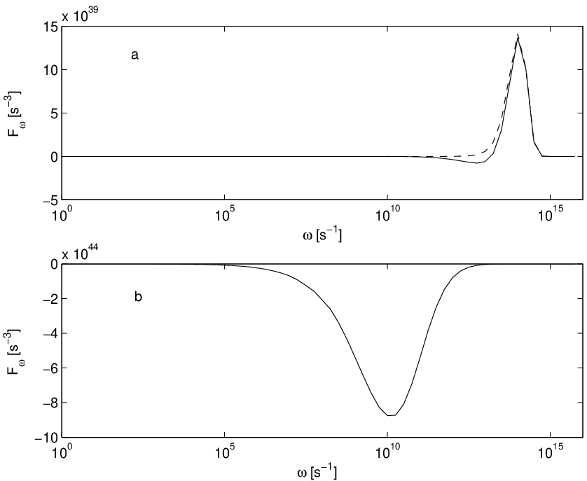
In 1, a net deviation from the zero-temperature value of the Casimir force is predicted to be about 25% for a plate separation of m at 300 K. The experimental results reported in 2 had their greatest sensitivity around 1 m, and disagree significantly with the results in 1. As a comparison, we numerically integrate Eq. 2) for m and K, using Eq. (5) for the permittivity. The results are shown in Fig. 1, where we have separated the results from the two integration paths. In Fig. 1a, it can be seen that there is no significant deviation from the perfectly conducting case. On the other hand, the contribution from evanescent waves, shown in Fig. 1b, is large and the integrated value is in good agreement with the result given in 1.
We see immediately that the main contributions of the -mode finite conductivity correction are around s-1. This behavior is due to an approximately quadratic increase with of the integral and a suppression beginning at s-1 due to . This is a low frequency range and we can question certain assumptions in 1 and in the Lifshitz calculation, among others, in regard to theoretical predictions relevant to the experimental arrangement in 2.
III Low Frequency Limit and Field Behavior in Metallic Materials
When the depth of penetration of the electromagnetic field into a metal,
| (6) |
where is the conductivity and is the permeability (for Au and Cu, , ), becomes of the same order as the mean free path of the conduction electrons, it is no longer possible to describe the field in terms of a dielectric permeability 12; 13. This occurs for optical frequencies s-1 for metals such as Au and Cu where the mean free path, at 300 K, is about cm 14 (p. 259). At frequencies above s-1 the permeability description again becomes valid because on absorbing a photon, a conduction electron acquires a large kinetic energy and has a shortened mean free path. However, in the interaction of a field with a material surface, and can always be related linearly through the surface impedance (which relates the electric field at the surface to a surface current hence magnetic field); this approach has been used in calculation of the Casimir force 15. A related correction arises from the the plasmon interaction with the surface which becomes significant near the plasma frequency of the metal, and has been estimated as nearly 10% 16 for sub-m plate separations.
The proper boundary conditions for a conducting plane have been discussed by Boyer 17. He points out that when (using here the notation of 1) , where is the resistivity and is the dissipation, the usual dielectric boundary conditions are not applicable. For Au, using the parameters in 1, this limit is met for . This corresponds to an optical wavelength of 5 m, which implies that for plate separations significantly larger than this, and of course for , the plates must be treated as good conductors.
The boundary conditions for a conducting surface are discussed in 18 (Sec. 8.1). At low frequencies (e.g., where the displacement current can be neglected), a tangential electric field at the surface of a conductor will induce a current , where is the conductivity. The presence of the surface current leads to a discontinuity in the normal derivative of , hence a discontinuity in the normal derivative of , at the boundary of a conducting surface. These boundary conditions are quite different from the dielectric case where the fields and their derivatives are assumed continuous.
These boundary conditions are applicable when the skin depth of the electromagnetic field is much smaller that the characteristic wavelength of the field. The wavelengths that contribute most to the Casimir force correspond to wavevector , independent of frequency, by numerical determination. When , the boundary conditions are applicable. This is well-satisfied over the entire frequency range of the finite temperature effect for the conditions of the experiment 2; when in which case m and the relationship, for m
| (7) |
at the lowest frequency of interest. In this frequency range, specifying the vector in the material as a boundary condition is not warranted.
This can also be understood by noting that the propagation of electromagnetic field in a conductive material is described by the diffusion equation. If we imaging a spatially periodic varying field on the surface of the material as , the variations propagate into the material, damped exponentially as into the material, where is interpreted as the diffusion length. We therefore see that over the frequency range of interest, the conducting boundary conditions are appropriate. In this limit, the displacement current is small compared to the real current, , for good conductors of interest here.
IV Electromagnetic Modes between Metallic Plates
We are interested in modes between two conducting plates separated by a distance . In the limit that the plates are thin films of thickness , the skin depth, we can assume that the plates are infinitely thick and the problem is considerably simplified. This is valid for the experiment 2 where the Cu/Au metallic film was 1 m. Essentially all of the mode thermal correction comes in the and s-1 range as shown in Fig. 1, so m.
Taking the axis as perpendicular to the plates, and the mode propagation direction along , for the case of modes (also referred to as or magnetic modes), . The plates surfaces are located at and . For a perfect conductor, at the conducting surfaces. A finite conductivity makes this derivative non-zero, and can be estimated from the small electric field that exists at the surface of the plate, (see 18, Sec. 8.1 and Eq. (8.6)),
| (8) |
where and it is assumed that the displacement current in the metal plate can be neglected (), and that the inverse of the mode wavenumber is less than . and are related through Maxwell’s equation . Assuming a time dependence of , and vacuum between the plates,
| (9) |
where indicates sign of at and respectively. The boundary conditions at the surfaces are thus
| (10) |
Solutions of the form , where and is the transverse wavenumber, can be constructed for the space between the conducting plates. The eigenvalues can be determined by the requirement that Eq. (9) be satisfied at and . With the usual substitution , the eigenvalues are then given by (see 19, Sec. 7.2)
| (11) |
and the force can be calculated by the techniques outlined in 19, Sec. 7.3.
This result can be recast in the notation of the Lifshitz formalism, and the spectrum of the thermal correction can be calculated as before. Noting that ,
| (12) |
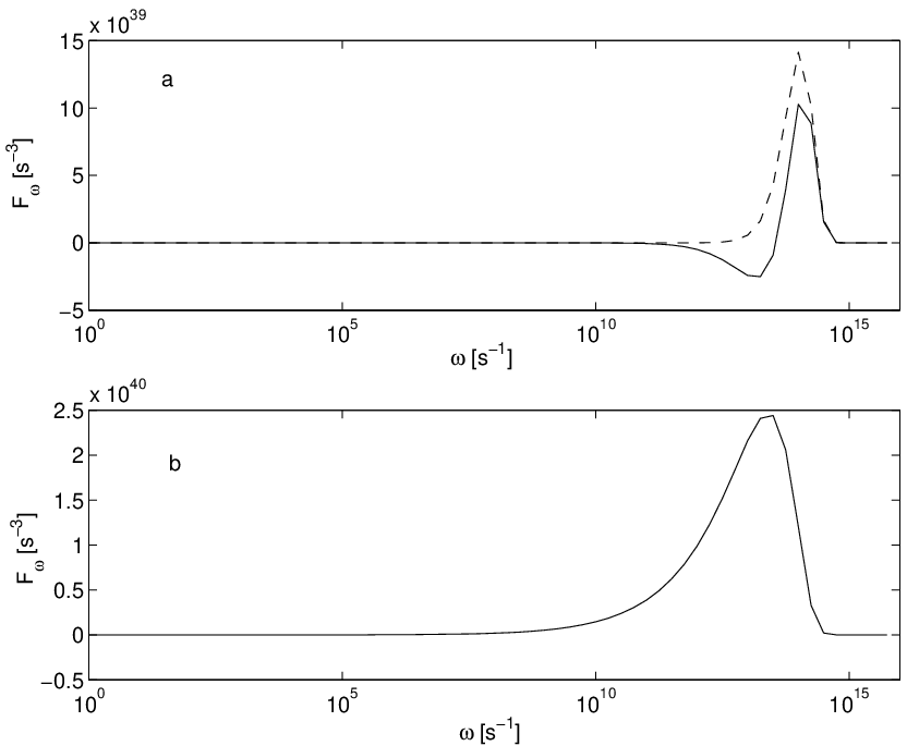
Results of a numerical integration are shown in Fig. 2, where it can be seen by comparison with Fig. 1 that the metallic plate boundary condition does not show a significant contribution from the integral of the mode thermal correction and is therefore similar to that for the “perfect conductor” boundary condition. This reconciles the discrepancy between the prediction in 1 and the experimental results reported in 2. Note that the function Eq. (11) in only applicable where the skin depth is small compared to the mode wavelength. Our result is in agreement, in its range of applicability, with the analysis presented in 15 which is valid for all frequencies. In this note, we essentially determined the surface impedance from the bulk properties, which is possible in over the frequency range of interest.
V Conclusion
The problem of calculating the mode contribution to the Casimir force has been previously treated with the “Schwinger prescription” 20 of setting the dielectric constant to infinity before setting . This prescription has become controversial 21, a term that can be used to describe the entire history of the theory of the temperature correction. However, there is no doubt that the issues brought up in 1 are important.
The purpose of our calculation is to take a different approach and to study the low-frequency behavior of the correction in order to understand its character. We have shown that the finite temperature correction in 1 is a low-frequency phenomenon. The frequency is sufficiently low so that treating the plates as bulk dielectrics is not valid. By use of a more realistic description of the field interaction with the plates we show that the modes between metallic plates of finite conductivity produce a finite temperature correction in close agreement with the perfectly conducting case. The principal difference between our result and the previous work is that we have allowed for the possibility that the derivatives of the fields at the conducting boundary are discontinuous. This possibility exists because the fields produce currents in the conducting plates that are discontinuous across the boundary between the vacuum and the conductor. Although it is tempting to model the finite conductivity as a modification to the dielectric permittivity, such a model fails when the mean free path of the conduction electrons exceeds the penetration depth of the electromagnetic field, and thus fails for frequencies of interest for the thermal correction to the electromagnetic mode.
We have shown that the conducting boundary conditions that are applicable for frequencies where the mode thermal correction has its significant contribution lead to a net increase of the mode force, and is of the same magnitude as the perfectly conducting case. This result is in agreement with the experimental results reported in 2. However, additional and improved experiments with large plate separations (greater than 2 m) with both conducting and dielectric plates would provide the definitive test. A particularly tempting dielectric would be diamond which offers both theoretical and experimental benefits: its dielectric properties can be calculated from first-principles, and stray surface charges can be eliminated by exposing it to ultraviolet light, making it photoconductive. A semiconductor such as lightly-doped Germanium would also provide a useful test of this theory. Ge with resistivity cm is readily available and would have a skin depth about 1,000 times that of Cu or Au. Additional high-accuracy measurements at long-range with Au or Cu are also important for testing the theory. We are presently constructing a new torsion pendulum system that will be able to measure the Casimir force with 1% accuracy at distances greater than 2 m, at a fixed temperature of 300 K. We hope that this note will spur further theoretical work on the questions and basic analysis presented here.
References
- (1) M. Böstrom and Bo E. Sernelius, Phys. Rev. Lett. 84, 4757 (2000).
- (2) S. K. Lamoreaux, Phys. Rev. Lett. 78, 5 (1997);81, 4549 (1998).
- (3) R.S. Decca et al., Phys. Rev. D 68, 116003 (2003).
- (4) S. K. Lamoreaux, Phys. Rev. Lett. 87, 139101 (2001).
- (5) M. Bordag et al. , Phys. Rev. Lett. 85, 503 (2000).
- (6) G. L. Klimchitskaya, Int. Jour. Mod. Phys. A 17, 751 (2002).
- (7) C. Genet, A. Lambrecht, and S. Reynaud, Int. Jour. Mod. Phys. A 17, 761 (2002).
- (8) Bo E. Sernelius and M. Böstrom,Phys. Rev. Lett. 87, 259101 (2001); I. Brevik, J. B. Aarseth,and J. S. Hoye, Phys. Rev. E 66, 026119 (2002).
- (9) J.S. Høye, I. Brevik, J.B. Aarseth, and K.A. Milton, Phys. Rev. E 67, 056116 (2003).
- (10) J.R. Torgerson and S.K. Lamoreaux, quant-ph/0208042.
- (11) B. Geyer, G.L. Klimchitskaya, and V.M. Mostepanenko, Phys. Rev A 67, 062102 (2003).
- (12) L. D. Landau and E. M. Lifshitz, Electrodynamics of Continuous Media (Pergamon, Oxford, 1960); Sec. 67.
- (13) L.H. Ford, Phys. Rev. A 48, 2962 (1993).
- (14) E.M. Lifshitz, JETP 2, 73 (1956).
- (15) H. London, Proc. Roy. Soc. A 176, 522 (1940).
- (16) C.H. Kittel, Solid State Physics (Wiley, N.Y., 1971).
- (17) R. Esquivel, C. Villarreal, and W.L. Mochàn, Phys. Rev. A 68, 52103 (2003).
- (18) T. H. Boyer, Phys. Rev. A 9, 68 (1974).
- (19) J. D. Jackson, Classical Electrodynamics, 2nd. Ed. (Wiley, NY, 1975).
- (20) Peter W. Milonni, The Quantum Vacuum (Academic Press, San Diego, 1994).
- (21) J. Schwinger, L. L. DeRaad, Jr. , and K. A. Milton,Ann. Phys. (New York) 115, 1 (1978).
- (22) K.A. Milton, The Casimir Effect: Physical Manifestations of Zero-Point Energy (World Scientific, Singapore, 2001); p. 54.