Interference as a statistical consequence
of conjecture on time quant
Abstract
We analyze statistical consequences of a conjecture that there exists a fundamental (indivisible) quant of time. We study particle dynamics with discrete time. We show that a quantum-like interference pattern could appear as a statistical effect for deterministic particles, i.e. particles that have trajectories and obey deterministic dynamical equations, if one introduces a discrete time. As a demonstration of this concept we consider particle scattering on a screen with a slit. We study how resulting interference picture depends on the parameters of the model. The resulting interference picture has a nontrivial minimum-maximum distribution which vanishes, as the time discreteness parameter goes to zero. This picture is qualitatively the same as one obtained in quantum experiments. The picture includes some interesting nonclassical properties such as a ‘black’ region behind the center of the slit.
1 Introduction
there exists a fundamental quant of time .
In fact we came to this conjecture by finding (by pure occasion) that statistical histograms obtained for classical systems in the one or two slit experiments can have the form of quantum-like interference observed in experiments with photons or electrons. We started to speculate that essential features of quantum statistics (at least some of them) could be obtained as a consequence of existence of time quant.
Basically speaking the idea of discretization is quite natural for physics. Indeed discretization of energy was exploited by Plank-Einstein ideas in order to explain such quantum phenomena as black body radiation, photo-electric effect, etc. On the other hand from the point of view of energy-time uncertainty relations discretization of time gives certain constraints to a (measured) energy of the system.
On the other hand by introducing discretized time one effectively changes the theoretical structure of the space-time on small distances11 1 In particular, this idea was exploited by p-adic space-time alternative[9, 10, 11, 12]. From this point of view it is rather natural to assume that a value of the discreteness parameter is of the order of Plank time . One could think of discretized time as a lack of information of where the particle is during the discretization period.
In this paper we study deterministic model for particle scattering on a screen with a single slit. Resulting interference picture has a nontrivial minimum-maximum distribution which is qualitatively the same as one obtained in quantum experiments. The interference pattern appears as a statistical effect of particles which have trajectories22 2 Cf. with Bohmian mechanics[16, 17]. The interference picture has no relation to ‘self-interference’ of particles, no wave-structure is involved into considerations. The basic source of interference is the discrete time scale used in our mathematical model: instead of Newton’s differential equations with continuous time evolution, we consider difference equations with discrete time evolution. Interference effect disappears as the time discreteness parameter goes to zero. The picture includes some interesting nonclassical properties such as a ‘black’ region behind the center of the slit33 3 We would like to thank G. Emch for an interesting question he asked on the ‘International Conference: Reconsideration of Foundations-2’ held in Växjö – whether it is possible to reproduce Fresnel-like phenomenon of a black region behind the center of the slit in the discrete time formalism – our answer now is yes (see section 5 for details)..
The paper is organized as follows. In the next section we provide basic ideas of the discrete time formalism and compare it with construction of quantum mechanics. In section 3 we write dynamical equations with discrete time and in section 4 we present them in intuitive form. In section 5 we apply the formalism to a particle scattering on a screen with a slit and study appearance and properties of the resulting interference picture. Finally, in the appendix we provide a detailed description of the numerical simulation performed, we list a Mathematica program which mirrors the original parallel C++ programm which we used to perform actual simulation.
We remind that recently it was suggested[4, 5, 6, 7, 8] that quantum mechanical interference rules could be explained using contextual transformations. This approach makes one think of a construction of physically reasonable model which produces interference resting on the classical rule of addition of probabilistic alternatives (extended with a notion of context). Our quantum-time approach could be considered as a candidate for such a model.
2 Basic Steps of the Approach
According to the principles of quantum mechanics in order to compute measurable quantities, in the simplest case, one has to perform the following steps[13, 14]. First, the form of classical and quantum equations of motion remains the same (we are talking about Heisinberg’s representation), although the dynamical variables are now noncommutative. Next, one has to add to the original initial conditions an extra one stating commutative properties of the canonical variables, like . At the last step one says that measurable quantities are eigenvalues of the dynamical variables. Here the second step introduces the Plank constant which distinguishes classical and quantum worlds. The noncommutative property of dynamical variables is the root of the fact that quantum particles can not have trajectories and introduction of quantum state implies the nondeterministic behavior of quantum systems.
In this note we tried to achieve the same results for measurable quantities as in quantum mechanics (at least in the part vastly supported by experiments), but trying to keep trajectories and deterministic behavior of particles. We follow steps similar to the above ones, but we keep the measurable quantities being real functions. Nevertheless, we have had to introduce the time discreteness parameter . We start from classical equations of motion with discrete time and postulate the canonical variables to be measurable.
3 Discrete Time Dynamics
In both classical and quantum mechanics a dynamical function evolves according to the following well known equation
| (1) |
where is a Hamiltonian of the system and in the right hand side is a Poisson bracket, either classical or quantum44 4 Poisson bracket in classical mechanics could be presented as (2) and in quantum mechanics it is a commutator .
In both classical and quantum dynamics the left hand side of (1) is the same, it contains a continuous time derivative
As it was mentioned in the previous section we are interested in construction dynamics with discrete time. This is done with the help of discrete derivative which is postulated to be
where is the discreteness parameter. This parameter is finite and is treated in the same way as Plank constant in quantum mechanical formalism. In particular if is small relative to dimentions of the system then classical approximation with continuous derivative should work well (although this could not be the case all the time in the same sense as there are examples when quantum formalism is reasonable even for macroscopic systems, for example in superfluidity).
Thus the discrete time dynamical equation is postulated to be
where is a real-valued function of real-valued dynamical variables and in the right hand side there is the classical Poisson bracket (see (2)).
Please note that in our model the coordinate space is left continuous.
4 Discrete Time in Newton’s Equations
In this section we provide an intuitive description of the discretization procedure described above. Consider a well known Newton’s equation
| (3) |
This equation gives the same dynamics as (1)-(2). Let us now modify this equation, introducing the time discreteness parameter . We rewrite the second order differential equation (3) as a system of first order differential equations, we have
| (4) |
In the system (4) the derivatives assume continuousness of time. Let us now introduce the discreteness parameter . We have
| (5) |
5 Interference Pattern in a Single Slit Scattering
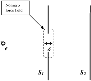
Consider the following experimental setup (see Fig.1). A particle source is located in front of the center of a slit in a screen . Near the slit there is a nonzero force field which affects particles,
( and are coordinates along horizontal and vertical axes respectively, the axes origin is in the center of the slit). Particles pass through the slit and concentrate on a second screen . We study a particle density on the screen .

Let us start from the simplest case when the force field is constant and perpendicular to the screens, , for and otherwise. Let the source be point-like emitting particles with constant velocity under random evenly distributed angles . In this case trajectories of particles emitted by (in discrete time dynamics) in the region (i.e. before the screen ) form concentric circles originating from with the radii , (Fig.2). We get the circles – which are trajectories of many particles emitted under close angles – in the region where there is no force field and particles move along strait lines, exactly as in classical dynamics. Let be the points where these circles enter the region . The distance between the center of the slit and is given by
| (7) |
where is a distance between and , and is the largest integral value not greater than a fraction ,
| (8) |
This rather simple setup already produces interesting nontrivial interference pattern (Fig.3).
The points are the origins of deviation from ‘classical’ (i.e. continuous time) trajectories. This deviation forms the interference pattern. To argument this let be an angle between the horizontal axis and a line connecting and . Particles emitted under angles less than () become affected by the force field in the region one step earlier than those emitted under angles grater than . As a result there appears a ‘fork’ – even very close trajectories but with the angles above and below become separated. One could get the points of minima of the interference pattern by following the trajectory along the line and the parabolic curve (movement in a constant field) in the region until the trajectory hits the screen .


The case described above is not completely physically reasonable, indeed is requires a force field everywhere in the half-plane , thus it could be considered only as a simplified model which still demonstrates some interesting properties of discrete time dynamics. An example of such a property is a Fresnel-like phenomenon of a black region behind the center of the slit which is discussed below.
One could see from (7)-(8) that if
then , and thus the particle trajectories emitted under positive and negative become separated. This forms a black region in the center of the screen just behind the slit (Fig.4).

Although we succeeded with a model of a field localized near the slit. We took Gaussian rapidly changing force field of the form
It is very stimulating that such setup also produces nontrivial pattern, since it means that one could start thinking of a physical nature of this force field.
We have also considered the case of non-point-like Gaussian source distributed along the vertical line. This produces smoother picture, which could be obtained by convolving the pattern on Fig.3 with a Gaussian kernel.
Acknowledgments
We would like to thank I would like to thank L. Accardi, L. Ballentine, V. Belavkin, G. Emch, B. Dragovich, R. Gill, D. Greenberger, K. Gustafsson, B. Hiley, G. t‘Hooft, L.V. Joukovskaya, A. Plotnitskii, I.V. Volovich for stimulating discussions on quantum phenomena.
References
- [1] A.Yu. Khrennikov, Ya.I. Volovich, Discrete Time Leads to Quantum-Like Interference of Deterministic Particles, in: Quantum Theory: Reconsiderations of Foundations, ed. A. Khrennikov, Växjö University Press, p. 455, quant-ph/0203009, (2002).
- [2] A.Yu. Khrennikov, Ya.I. Volovich, Interference effect for probability distributions of deterministic particles, in: Quantum Theory: Reconsiderations of Foundations, ed. A. Khrennikov, Växjö University Press, p. 441, quant-ph/0111159, (2001).
- [3] A.Yu. Khrennikov, Ya.I. Volovich, Discrete Time Dynamical Models and Their Quantum Like Context Dependant Properties, Proceedings of ‘Mysteries, Puzzles and Paradoxes in Quantum Mechanics - Garda 2003’, to appear in J.Mod.Opt. (2004).
- [4] Andrei Khrennikov, Linear Representations of Probabilistic Transformations Induced by Context Transitions, J. Phys.A: Math. Gen., 34, 9965-9981, (2001).
- [5] Andrei Khrennikov, Ensemble Fluctuations and the Origin of Quantum Probabilistic Rule, J. Math. Phys., 43 (2), 789-802, (2002).
- [6] Andrei Khrennikov, Representation of the Kolmogorov Model Having all Distinguishing Features of Quantum Probabilistic Model, Phys. Lett. A, 316, 279-296, (2003).
- [7] Andrei Khrennikov, Il Nuovo Cimento, B 115, N.2, pp. 179-184, (1999).
- [8] A. Khrennikov, Växjö interpretation of quantum mechanics, quant-ph/0202197, (2002).
- [9] V.S. Vladimirov, I.V. Volovich and E.I. Zelenov, -adic Analysis and Mathematical Physics, World Sci., (1994).
- [10] P. G. O. Freund and E. Witten, Adelic string amplitudes, Phys. Lett. B, 199, 191-195, (1987).
- [11] P. H. Frampton and Y. Okada, -adic string -point function, Phys. Rev. Lett. B, 60, 484-486, (1988).
- [12] A.Yu. Khrennikov, -adic Valued Distributions in Mathematical Physics, Kluwer Acad. Publ., Dordrecht, (1994).
- [13] W. Heisinberg, Über Quantentheoretische Undeutung kinematischer und mechanischer Beziehungen, Zs. Phys., 33, pp. 879-883, (1925).
- [14] W. Heisenberg, Physical principles of quantum theory, Chicago Univ. Press, (1930).
- [15] L. E. Ballentine, The statistical interpretation of quantum mechanics, Rev. Mod. Phys., 42, 358-381, (1970).
- [16] D. Bohm, Quantum theory, Prentice-Hall, Englewood Cliffs, New-Jersey, (1951).
- [17] D. Bohm and B. Hiley, The undivided universe: an ontological interpretation of quantum mechanics, Routledge and Kegan Paul, London, (1993).
Numerical Simulation
Here we provide a Mathematica program for computation of the histogram. Please note that although this program is approximately times slower than a more powerful parallel C++ program which we used to actually perform computations it reproduces the same results (in the simplest case where the computation time allowed us to wait the result) and could be seen as a detailed description of the numerical experiment which was performed as a demonstration of the concept.
ComputeTrajectory=Compile[{{, _Real}},
With[{
, (* Frame parameters *)
, (* Charge *)
, (* Discreteness parameter *)
(* Initial velocity *)
},
Module[{
},
While[,
;
;
;
;
;
;
];
Module[{
,
},
]]]];