Quantum Reversibility: Is there an Echo?

In this Letter we study the probability of return $P(t_{1},t_{2})$ for a generalized wavepacket dynamics scenario. The system is prepared in some initial state $\Psi_{\mbox{\tiny prep}}$, which can be regarded as the outcome of a preparation procedure which is governed by a Hamiltonian ${\cal H}_{\mbox{\tiny prep}}$. We assume that the quantum mechanical evolution is generated by Hamiltonians with classically chaotic limit: The state is propagated for a time $t_{1}$ using a Hamiltonian ${\cal H}_{1}$, and then the evolution is time-reversed for a time $t_{2}$ using a perturbed Hamiltonian ${\cal H}_{2}$. The corresponding evolution operators are $U_{1}$ and $U_{2}$. The probability of return to the initial state is

There are two special cases that have been extensively studied in the literature. The traditional wavepacket dynamics scenario H91 is obtained if we set $t_{2}=0$. In this context the “survival probability” is defined as

The “Loschmidt echo” (LE) scenario is obtained if we set $t_{1}=t_{2}=t$. In this context the “fidelity” is defined as

The theory of the fidelity was the subject of intensive studies during the last 3 years P84; JP01; JSB01; CT02; PS02; BC02; WC02; PLU95; VH03. It has been adopted as a standard measure for quantum reversibility following P84 and its study was further motivated by the realization that it is related to the analysis of dephasing in mesoscopic systems Z91.

In the present Letter we consider the full scenario of a time reversal experiment. The probability to find the system in its original state is $P(t)=P(t,0)$ before the time reversal ($t<T/2$), and

after the time reversal ($t>T/2$). The period $T$ is the total time of the experiment. The naive expectation, which is also reflected in the term “Loschmidt echo”, is to have a maximum for $P(t)$ at the time $t=T$. We are going to show that this expectation is wrong. We find that the maximum return probability is obtained at a time $t_{r}$ which in general is shorter than that. Namely,

If we have $t_{r}=T/2$ we say that there is no reversibility. If we have $t_{r}\sim T$ we say that we have a nearly perfect echo. We show that $t_{r}/T$ is a function of a dimensionless parameter $0<\lambda<\infty$. Namely,

where $\varepsilon_{\mbox{\tiny prep}}$ quantifies the difference between the evolution Hamiltonian ${\cal H}$ and the preparation Hamiltonian ${\cal H}_{\mbox{\tiny prep}}$, while $\varepsilon_{\mbox{\tiny evol}}$ quantifies the difference between the two instances ${\cal H}_{1}$ and ${\cal H}_{2}$ of the evolution Hamiltonian, which are used for the forward and for the time-reversed evolution respectively. The idea is that there is no way to have a complete control over the parameters (fields) of the systems. Therefore there is an unavoidable difference ($\varepsilon_{\mbox{\tiny evol}}$) between these two instances of ${\cal H}$, which by the setup of the experiment are regarded as identical. The scaling function (6) takes the limiting value $f(0)=1$ (echo) while for $\lambda>\lambda^{*}$ we get $f(\lambda)=0.5$ (no reversibility). Here $\lambda^{*}$ is some system-specific constant of order unity.

The most popular preparation which is considered in the literature, either in the context of wavepacket dynamics or fidelity (LE) studies, is a Gaussian wavepacket. Obviously the choice of such preparation is motivated mainly by the wishful thinking of theoreticians. However, in many applications, one is not so much interested in evolving an initial Gaussian wavepacket. This is certainly the situation in quantum information processing NC00 and in spin-echo experiments PLU95 where one starts with a random initial state. Formally a Gaussian wavepacket can be regarded as the ground state of a phase-space shifted Harmonic oscillator. Therefore it is characterized by a very large $\varepsilon_{\mbox{\tiny prep}}$, leading to $\lambda\ll 1$. In this Letter we do not assume $\lambda\ll 1$, but rather consider the general case.

In order to develop a general theory we need a model in which we have control over both $\varepsilon_{\mbox{\tiny prep}}$ and $\varepsilon_{\mbox{\tiny evol}}$. We consider a quantized system whose classical analog has positive Lyapunov exponent. Its Hamiltonian ${\cal H}={\cal H}(Q,P;x)$ depends on a parameter (field) variable $x$ which is determined by the experimental setup. For example it can be either a gate voltage or a magnetic flux. The dynamics takes place within a classically small (but quantum mechanically large) energy window. The classical dynamics is assumed to have a well defined finite correlation time $\tau_{\rm cl}$. We consider classically small (but possibly quantum mechanically large) perturbations ($x\mapsto x+\delta x$). Accordingly, the Hamiltonian can be linearized as follows:

We define ${\cal H}_{1}$ and ${\cal H}_{2}$ by setting $\delta x=\pm\varepsilon_{\mbox{\tiny evol}}$. The requirement of having classically small $\delta x$ means that the phase space structure of ${\cal H}_{1}$ and ${\cal H}_{2}$ is similar, and that any (small) difference in the chaoticity can be neglected. (we have verified that this smallness condition is satisfied for the example below).

The preparation issue requires further discussion. The traditional possibility is to prepare a Gaussian wavepacket (also known as a coherent state preparation). We regard this possibility as uncontrolled because the value of $\varepsilon_{\mbox{\tiny prep}}$ is ill defined. To have a physically meaningful definition of $\varepsilon_{\mbox{\tiny prep}}$ the natural procedure is as follows: We define a preparation Hamiltonian ${\cal H}_{\mbox{\tiny prep}}$ by setting $\delta x=\varepsilon_{\mbox{\tiny prep}}$. Then we start with an initial eigenfunction of ${\cal E}$, and evolve it with ${\cal H}_{\mbox{\tiny prep}}$ until we get an ergodic-like steady state within an energy shell (note rmrk). The width of this energy shell is proportional to $\varepsilon_{\mbox{\tiny prep}}$. The resulting wavepacket is used as an initial state for the time reversal experiment. For the purpose of comparison we shall consider also a Gaussian wavepacket preparation. For such preparation $\lambda\ll 1$ irrespective of its energy width. The reason is that this preparation does not occupy ergodically its energy shell. Formally one can say that for a Gaussian wavepacket ${\cal H}_{\mbox{\tiny prep}}$ differs enormously from the evolution Hamiltonian. There is no point in quantifying this difference. This is the reason why we use our controlled preparation procedure, where ${\cal H}_{\mbox{\tiny prep}}$ differs from the evolution Hamiltonian in a well defined manner. In any case we shall verify that a Gaussian wavepacket is indeed like taking a preparation with $\lambda\ll 1$.

In our numerical investigation we use the model Hamiltonian

with $x=1+\delta x$. It describes the motion of a particle in a 2D well (2DW). The physical units are chosen so as to have dimensionless variables. Therefore upon quantization the Planck constant $\hbar$ is a dimensionless quantity. Our numerical study is focused on an energy window around $E\approx 3$ where the motion is mainly chaotic with characteristic correlation time $\tau_{\rm cl}\approx 1$ CK01. The quantization is done with $\hbar=0.012$. We write the Hamiltonian matrix as in Eq. (7), using a basis such that ${\cal E}$ is diagonal. The mean level spacing is $\Delta\approx 4.3\times\hbar^{2}$. As expected, on the basis of a general “quantum chaos” argumentation FP86, the matrix ${\cal B}$ is a banded matrix. More details regarding the band profile can be found in Ref. CK01. The only additional piece of information that is needed for the following analysis is the parametric scale $\delta x_{c}$. This is defined as the $\delta x$ which is needed in order to mix neighboring levels. It is given by the ratio $\Delta/\sigma$, where $\sigma$ is the root mean square value of the near diagonal matrix elements of the ${\cal B}$ matrix. For the above model $\delta x_{c}\approx 3.8*\hbar^{3/2}$.

Fig. 1 (left panel) displays representative results of simulated time reversal experiments. One experiment is done with a coherent state preparation, and we indeed see behavior that looks like an echo ($t_{r}\sim T$). Qualitatively the same behavior is observed for a random preparation that has $\lambda\ll 1$. Once we take a preparation with a larger value of $\lambda$, we realize that the compensation time is in general $t_{r}<T$. In particular with the $\lambda>1$ preparation we do not observe any quantum reversibility ($t_{r}=T/2$).

In Fig. 2 we present some results for $t_{r}/T$. We clearly see that $t_{r}$ is smaller for larger values of $\varepsilon_{\mbox{\tiny evol}}$. Much more illuminating is Fig. 3 where we present our numerical results for $t_{r}$ and various $T$. The points corresponding to the same $\lambda$ but different values of $\varepsilon_{\mbox{\tiny evol}}$ and $\varepsilon_{\mbox{\tiny prep}}$ fall onto the same smooth curve with a good accuracy, confirming the scaling hypothesis (6). Moreover, we see that for $\lambda>\lambda^{*}$, with $\lambda^{*}\approx 1.3$, we have $t_{r}=T/2$ (no echo) irrespective of the actual value of $\varepsilon_{\mbox{\tiny prep}}$ and $\varepsilon_{\mbox{\tiny evol}}$. Thus, if we want a $\lambda>\lambda^{*}$ type of preparation, we simply can set $\varepsilon_{\mbox{\tiny prep}}=0$, which means an eigenstate of ${\cal E}$. From Fig. 3 we also see that in the other limiting case of $\lambda\ll 1$ we have (nearly) an echo. This is the same as in the case of a Gaussian wavepacket preparation.

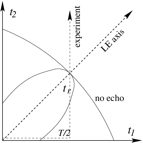
In order to explain the observed results for $t_{r}$ we look on Fig. 4. There are two axes along which the theory of $P(t_{1},t_{2})$ is quite well known. One is the traditional wavepacket dynamics axis $t_{2}=0$ along which $P_{\mbox{\tiny SR}}(t)$ is defined, while the other is the “LE axis” ($t_{2}=t_{1}$) along which $P_{\mbox{\tiny LE}}(t)$ is defined. In the figure we also indicate the course of a time reversal experiment. It is clear that in order to have $t_{r}<T$ the contor line $P(t_{1},t_{2})=P_{\mbox{\tiny SR}}(T/2)$ should meet the $t_{1}$ axis in a sharp angle. Furthermore, if we want to have some remnant of an echo at the end of the period ($t=T$) we have to cross the contour line $P(t_{1},t_{2})=P_{\mbox{\tiny LE}}(T/2)$. The condition for that is

In the following discussion we would like to assume that both $\varepsilon_{\mbox{\tiny prep}}$ and $\varepsilon_{\mbox{\tiny evol}}$ are larger than $\delta x_{c}$, which means that the perturbations are strong enough to mix levels. In such case the decay of $P_{\mbox{\tiny SR}}(t)$ or $P_{\mbox{\tiny LE}}(t)$ is approximately exponential:

Moreover in both cases $\gamma$ is given by the expression

where $\gamma_{\mbox{\tiny PT}}$ is the value which is determined by perturbation theory, while $\gamma_{\mbox{\tiny SC}}$ is determined by semiclassical considerations.

Once details are concerned the theory behind the exponential approximation Eq. (10) becomes quite different in the two respective cases [$P_{\mbox{\tiny SR}}(t)$, $P_{\mbox{\tiny LE}}(t)$]. The theory of the survival probability is related to the parametric theory of the LDOS CH00; CK01. Namely, for relatively small perturbations $\gamma=\gamma_{\mbox{\tiny PT}}\propto(\varepsilon_{\mbox{\tiny prep}}/\delta x_{c})^{2}$ is essentially the width of Wigner’s Lorentzian, while for large perturbations $\gamma=\gamma_{\mbox{\tiny SC}}\propto\varepsilon_{\mbox{\tiny prep}}$ is the width of the energy shell (in the latter case the exponential approximation is at best a good fit). In contrast to that, the theory of the fidelity $P_{\mbox{\tiny LE}}(t)$ is related to a theory of dynamical correlations, and cannot be reduced to the LDOS analysis WC02. The best theory to date is semiclassical (see  VH03 and references therein). As in the case of the survival probability we have $\gamma=\gamma_{\mbox{\tiny PT}}\propto(\varepsilon_{\mbox{\tiny evol}}/\delta x_{c})^{2}$ for small perturbations, while for large perturbations $\gamma=\gamma_{\mbox{\tiny SC}}$, in some typical cases, is related to the Lyapunov exponent. We would like to point out that the study of the general conditions for having a fingerprint of the Lyapunov exponent in time reversal experiments is still an open issue for future study HKC03. The existing semiclassical theory for the “echo” phenomena assumes Gaussian wavepackets.

By definition $P_{\mbox{\tiny SR}}(T/2)$ depends only on $\varepsilon_{\mbox{\tiny prep}}$, while $P_{\mbox{\tiny LE}}(T/2)$ is mainly sensitive to $\varepsilon_{\mbox{\tiny evol}}$. Therefore it is evident that a small $\lambda$ is a condition for having $t_{r}<T$. If we have $\lambda\ll 1$ then the contour line $P(t_{1},t_{2})=P_{\mbox{\tiny LE}}(T/2)$ can be very close to the LE-axis. This implies that for $\lambda\ll 1$ we can get nearly a perfect echo behavior ($t_{r}\sim T$). This picture, as we have seen before, is supported by our numerical findings.

As we have seen above, the applicability of semiclassical considerations is not essential for having an “echo”. The general picture that we have outlined should be valid also in the absence of a semiclassical limit. This is in contrast to the impression that one might get from the recent literature. In order to establish this provocative statement, in a way that leaves no doubts, we use a simple random matrix theory (RMT) procedure. We take the resulting banded matrix ${\cal B}$ of the 2DW model (8), and randomize the signs of the off-diagonal terms. In this way we get an effective RMT (ERMT) model of the type that had been introduced by Wigner 50 years ago wigner. The model is characterized by the same mean level spacing, and by the same band-profile as the physical 2DW model. Consequently the generated dynamics is characterized by the same correlation time (the latter is determined by the bandwidth). But unlike the 2DW model, the ERMT model is lacking a semiclassical limit. In the right panels of figures 1-3 we demonstrate the results of simulations that were done with the ERMT model. We clearly see that we get similar results (in Fig.3 the RMT drop is slightly sharper).

In summary, we have shed a new light on the physics of quantum reversibility, and in particular we have introduced the concept of compensation time $t_{r}$, which replaces the misleading terminology of “echo”. Our predictions should be tested in wave field evolution experiments such as spin polarization echoes in nuclear magnetic resonances PLU95; prv. In particular we have considered the realistic case of a general preparation, and clarified the role of semiclassical considerations in the theory.

It is our pleasure to thank Horacio Pastawski and Bilha Segev (BGU) for useful discussions. This research was supported by the Israel Science Foundation (grant No.11/02), and by a grant from the GIF, the German-Israeli Foundation for Scientific Research and Development.

References

- (1) E. J. Heller, Chaos and Quantum Systems, edt. M.-J. Giannoni et al. (Elsevier, Amsterdam), (1991)
- (2) A. Peres, Phys. Rev. A 30, 1610 (1984).
- (3) R.A. Jalabert and H.M. Pastawski, Phys. Rev. Lett. 86, 2490 (2001); F.M. Cucchietti, H.M. Pastawski, R. Jalabert Physica A, 283, 285 (2000); F.M. Cucchietti, H.M. Pastawski and D.A. Wisniacki Phys. Rev. E 65, 046209 (2002);
- (4) Ph. Jacquod, I. Adagdeli and C.W.J. Beenakker, Phys. Rev. Lett. 89, 154103 (2002); Ph. Jacquod, I. Adagdeli and C.W.J. Beenakker, Europhys. Lett. 61, 729 (2003); Ph. Jacquod, P.G. Silvestrov and C.W.J. Beenakker, Phys. Rev. E 64, 055203(R) (2001).
- (5) N.R. Cerruti and S. Tomsovic, Phys. Rev. Lett. 88, 054103 (2002); J. Phys. A: Math. Gen. 36, 3451 (2003).
- (6) T. Prosen, Phys. Rev. E 65, 036208 (2002); T. Prosen and M. Znidaric, J. Phys. A: Math. Gen 35, 1455 (2002); ibid 34, L681 (2001); T. Prosen and T. H. Seligman, ibid 35, 4707 (2002); T. Kottos and D. Cohen, Europhys. Lett. 61, 431 (2003).
- (7) G. Benenti and G. Casati, Phys. Rev. E 66, 066205 (2002); W. Wang and B. Li, ibid. 66, 056208 (2002).
- (8) D. A. Wisniacki and D. Cohen, ibid. 66, 046209 (2002).
- (9) Jiri Vanicek and Eric J. Heller, quant-ph/0302192.
- (10) H. M. Pastawski, P. R. Levstein and G. Usaj, Phys. Rev. Lett. 75, 4310 (1995); G. Usaj, H. M. Pastawski and P. Levstein, Molecular Physics 95, 1229 (1998).
- (11) W. H. Zurek, Phys. Today 44, 36 (1991); D. Cohen and T. Kottos cond-mat/0302319; D. Cohen, Phys. Rev. E 65, 026218 (2002).
- (12) M. A. Nielsen and I. L. Chuang, Quantum Computation and Quantum Information (Cambridge University Press, 2000).
- (13) Doron Cohen, and Tsampikos Kottos, Phys. Rev. E, 63 36203, (2001).
- (14) M. Feingold and A. Peres, Phys. Rev. A 34 591, (1986); M. Feingold, D. Leitner, M. Wilkinson, Phys. Rev. Lett. 66, 986 (1991); M. Feingold, A. Gioletta, F. M. Izrailev, L. Molinari, ibid. 70, 2936 (1993); M. Wilkinson, M. Feingold, D. Leitner, J. Phys. A 24, 175 (1991).
- (15) Doron Cohen, and E. J. Heller, Phys. Rev. Lett. 84 2841, (2000).
- (16) M. Hiller, T. Kottos and D. Cohen, in preparation (2003).
- (17) E. Wigner, Ann. Math 62 548 (1955); 65 203 (1957); V.V. Flambaum, A.A. Gribakina, G.F. Gribakin and M.G. Kozlov, Phys. Rev. A 50 267 (1994); G. Casati, B.V. Chirikov, I. Guarneri, F.M. Izrailev, Phys. Rev. E 48, R1613 (1993); Phys. Lett. A 223, 430 (1996); Ph. Jacquod and D. L. Shepelyansky, Phys. Rev. Lett. 75, 3501 (1995); Y. V. Fyodorov, O. A. Chubykalo, F. M. Izrailev, and G. Casati, ibid. 76, 1603 (1996).
- (18) H. M. Pastawski, private communication.
- (19) To ensure phase space (semiclassical) ergodicity of the wavefunction within the energy shell we randomize the signs of the state vector elements in the basis.