Spin-dependent Bohm trajectories for hydrogen eigenstates
Abstract
The Bohm trajectories for several hydrogen atom eigenstates are determined, taking into account the additional momentum term that arises from the Pauli current. Unlike the original Bohmian result, the spin-dependent term yields nonstationary trajectories. The relationship between the trajectories and the standard visualizations of orbitals is discussed. The trajectories for a model problem that simulates a - transition in hydrogen are also examined.
1 Introduction
In David Bohm’s original causal interpretation of quantum mechanics [1], the motion of a quantum mechanical particle is determined by its wavefunction , which acts as a guidance wave [3]. If the wavefunction is written as
| (1) |
where and and are real-valued, then the trajectory of the particle is determined by the relation
| (2) |
The Schrödinger current associated with is given by
| (3) |
where . Comprehensive discussions of this causal interpretation of quantum mechanics can be found in [2] and [7].
However, as Holland [8] has pointed out, Eqs. (2) and (3) are relevant only to spin-0 particles. For particles with spin, these equations are inconsistent if the theory is to be ultimately embedded in a relativistic theory. The condition of Lorentz covariance on the law of motion implies that the momentum of a particle with spin s must be given by [8]
| (4) |
In a number of earlier works, including [4, 5, 6], the current vector associated with Eq. (4),
| (5) |
was referred to as the Pauli current, the nonrelativistic limit of the Dirac current, as opposed to Eq. (3), the nonrelativistic limit of the Gordon current. (In these papers, it was claimed that consistency with Dirac theory requires that Schrödinger theory be regarded as describing an electron in an eigenstate of spin.) The spin-dependent term was also discussed in [2] but only in the context of the Pauli equation and not the Schrödinger equation.
The momentum defined in Eq. (2) predicts that electrons in an eigenstate are stationary since . This is a counterintuitive result of Bohm’s original theory, but one which no longer persists when the extra term in (4) is taken into account. For example, consider an electron in the the ground eigenstate of hydrogen,
| (6) |
where is the Bohr radius. Also assume that the electron is in a definite spin eigenstate: Without loss of generality, let its spin vector be given by . (We shall justify this assumption below.) Holland [7] showed that the extra term implies that the polar coordinates and are constant, with angle evolving in time as follows:
| (7) |
All points on a sphere of radius orbit the -axis at the same rate. If , the angular frequency is on the order of , cf. Eq. (32).
In Section 2, we examine the effects of the extra term in (4) for an electron in several eigenstates of the hydrogen atom. Because the momentum equation (4) now involves spin, a complete description of the electron in the atom – provided by an appropriate wavefunction – will have to involve both spatial as well as spin information. Let us denote the complete wavefunction of the electron by , where denotes appropriate spin coordinates. Since the hamiltonian describing the evolution of is the simple spin-independent hydrogen atom hamiltonian , we may write as the tensor product , where is a solution of the time-dependent Schrödinger equation,
| (8) |
and is an eigenfunction of the commuting spin operators and , with and . Thus defines the “alpha” or “spin up” state to which corresponds the spin vector . As such, the remainder of our discussion can focus on the evolution of the spatial portion of the wavefunction . In the parlance of “state preparation,” one can view this construction as preparing the electon with constant spin vector and initial wavefunction . Given an initial position of the electron, Eq. (4) will then determine its initial momentum , from which its causal trajectory then evolves.
In Section 3, we examine the trajectories of an electron, as dictated by Eq. (4), where is a linear combination of and eigenstates evolving in time under the hydrogen atom hamiltonian, cf. Eq. (8). Once again because of the spin-independence of , we may assume that the spin vector of the elctron is constant, i.e., , and thereby focus on the time evolution of the spatial wavefunction . This simple model was chosen to determine the major qualitative features of Bohmian trajectories for a - transition induced by an oscillating electric field. We have analyzed trajectories corresponding to the time-dependent wavefunction associated with the transition hamiltonian and shall report the results elsewhere.
2 Spin-dependent trajectories of electrons in hydrogen eigenstates
2.1 Qualitative features
Following the discussion at the end of the previous section, we consider an electron with spin vector that begins in a hydrogenic eigenstate, i.e., . The time evolution of the spatial wavefunction is simply
| (9) |
Comparing Eqs. (9) and (1), we see that for a real eigenstate, so that the momentum in Eq. (4) is given by
| (10) |
Some simple qualitative information about the electron trajectories is readily found from this equation. First, the vector points in the direction of the steepest increase in , hence in . Because of the cross product, the momentum vector p is perpendicular to this direction. In other words, the trajectories of the electron lie on level surfaces of . However, p is also perpendicular to the direction of the spin, assumed to lie along the -axis in this discussion. This implies that z is constant for these Bohm trajectories.
From the above analysis, the shape of the Bohm trajectories may be found by computing level surfaces of – or simply for real-valued eigenfunctions – and then finding the intersections of these surfaces with planes of constant . An electron in the state of hydrogen, cf. Eq. (6), must therefore execute a circular orbit about the -axis. However, the angular velocity of this orbit, cf. Eq. (7), cannot be determined from this analysis.
For the case, with quantum numbers , the wavefunction is given by
| (11) |
The level surfaces of are spheres whose intersection with planes of constant are circles (with constant values). The electron again travels about the -axis in a circular orbit.
In the case, , the wavefunction is given by
| (12) |
The condition that both and be constant is satisfied only if both and are constant, once again yielding circular orbits about the -axis.
In the other cases, , the wavefunctions are given by
| (13) |
The condition yields a relation defined implicitly by
| (14) |
where is a constant. Since is also constant, it follows that both and are constants of motion so that there is circular motion about the -axis.
2.2 More detailed dynamical descriptions of the trajectories
For more complicated hydrogen eigenstates (see below), it may not be as simple to find closed form expressions for level sets of so that the method of qualitative analysis outlined above may be difficult if not impossible. As well, it is desirable to extract quantitative information such as the angular velocity of the circular orbits deduced earlier. We therefore analyze the differential equations of motion defined by Eq. (10).
The gradient term from Eq. (10) is given by
| (15) |
For real wavefunctions, this simplifies to
| (16) |
In spherical polar coordinates , the spin vector is given by . It is convenient to compute the cross product in the (right-handed) spherical polar coordinate system:
| (17) |
For the ground state defined in Eq. (6), . Thus
| (18) |
Since , it follows that and are constant, implying that is constant, i.e., circular orbits about the -axis. Holland’s result in Eq. (7) follows.
For the wavefunction defined in Eq. (11),
| (19) |
so that
| (20) |
Once again and are constant. From the relation , we have
| (21) |
Note that the pole at coincides with the zero of the wavefunction, implying that the probability of finding the electron at is zero. Also note that (i) for , (ii) for , (iii) for and (iv) for . For , the angular velocity is equal to that of the ground state, cf. Eq. (7).
For the state defined in Eq. (12),
| (22) |
From Eq. (10),
| (23) |
implying that
| (24) |
This is one-half the angular velocity for the ground state.
For the states with , cf. Eq. (13), is not identically zero and so we must use the momentum equation (4). We find that
The coordinates and are constant, implying circular orbits about the -axis. The orbital angular velocity is given by
It will be instructive (for an analysis of Eq. (29) below) to examine the Bohm trajectories resulting from Eq. (10), i.e. ignoring the term. We find that
| (25) |
Once again, and are constant, implying circular orbits about the -axis. However the orbital angular velocity depends upon and in a more complicated fashion:
| (26) |
For , i.e., the plane, for . This implies that there is a ring of equilibrium points on the plane at which the electron is stationary. For all other nonzero values on the plane the electron revolves about the -axis: for and for . A ring of stationary points exists on every plane parallel to the plane: For any fixed , the ring is determined by the relation . The radius of this ring (distance from the -axis) is . The set of all points at which the electron is stationary defines a surface that is generated by revolving the curves
| (27) |
about the -axis. In the region between this surface and the -axis, ; on the other side of this surface, .
In summary, for each of the hydrogen eigenstates studied above, the Bohm trajectories are circular orbits about the -axis, the assumed orientation of the electron spin vector . Furthermore, the quantitative behaviour of the angular velocity has been determined in all cases.
We now examine Bohm trajectories for the real hydrogen wavefunctions, [9]
| (28) |
where . The probability distributions associated with these wavefunctions are the familiar hydrogen orbitals used in descriptions of organic chemical bonding.
The and wavefunctions are obtained by appropriate linear combinations of the energetically degenerate eigenfunctions of Eq. (13). Therefore they are also eigenfunctions of the hydrogen atom hamiltonian with energy . From Eq. (9), it follows that . The cross product of Eq. (10) has components in all three variables, resulting in a system of three coupled ordinary differential equations which must be integrated to find the trajectories.
The system of ODEs associated with the wavefunction is given by
| (29) |
Note that the DE is identical to Eq. (25). From the first two DEs, we have
| (30) |
which is easily integrated to give , in agreement with our earlier analysis. It follows that and are constant when or . If as well, then for , implying the existence of two equilibrium points at and . At these points, the electron is stationary. In fact, these are two particular cases of an infinity of equilibrium points that are given by the conditions ( plane) and
| (31) |
By virtue of the above relation and Eq. (25), the equilibrium points of this system lie on the two curves defined by Eq. (27) in the plane as well as their reflections about the -axis. Each of these points corresponds to the points of highest and lowest “elevation” (from the horizontal plane) of the familiar dumb-belled level surfaces of the orbital. At all of these points, the electron is stationary.
The system of ODEs in (29) may be integrated numerically. However, it is useful to introduce the dimensionless variables and , where
| (32) |
is the angular frequency associated with the to transition in the hydrogen atom (). The scaled equations become
| (33) |
Figure 1 shows the numerically integrated trajectories for several initial conditions in the plane. Note that there is a good qualitative agreement between these trajectories and the orbital shapes of the state as depicted in textbook contour plots. (No orbits cross the plane since it is a nodal surface.) The numerical results confirm that motion is periodic. Angular frequency values are observed to be of the order of . These periodic orbits are stable in the sense of Lyapunov.
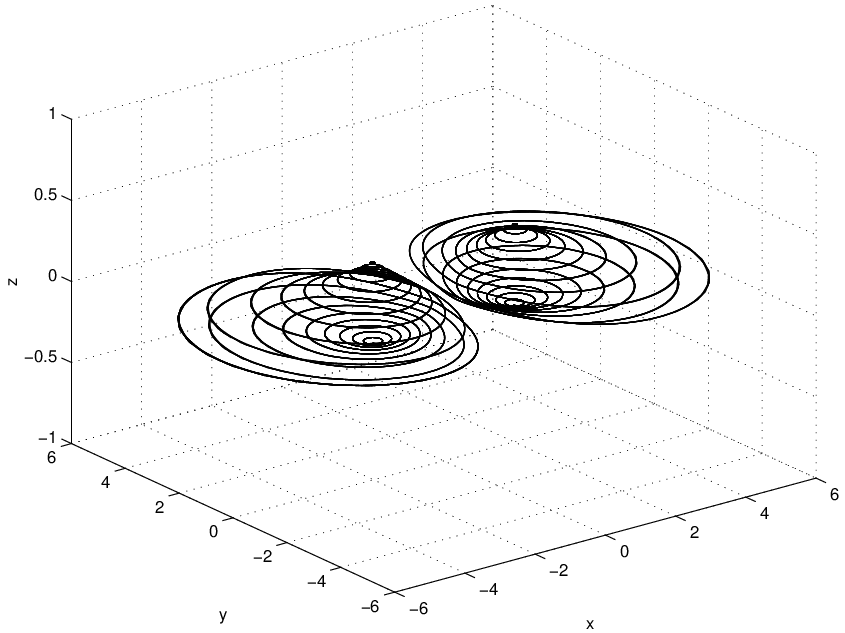
The nondimensional and numerical analysis of the case proceeds in a similar fashion. The resulting system of ODEs represents a rotation of the system in Eq. (29) by an angle of in .
To summarize this section, we have shown that the spin-dependent Bohm trajectories for the ground and first excited states of the hydrogen atom are stable periodic orbits. There are no exceptional orbits that deviate from this regularity. For some of the states, these orbits include families of stationary points that have zero Lebesgue measure in . These results are intuitively more acceptable than the original Bohmian result that all trajectories associated with a given eigenstate are stationary.
3 Trajectories associated with a linear superposition of hydrogenic eigenfunctions
We now examine the Bohm trajectories of an electron with constant spin vector but with a spatial wavefunction that begins as a linear combination of and hydrogenic eigenfunctions,
| (34) |
where . (The assumption that the electron is in a well-defined “spin up” eigenstate was justified at the end of Section 1.)
The time evolution of this spatial wavefunction, as dictated by the time-dependent Schrödinger equation (8), will be given by
| (35) |
This linear combination was chosen in order to examine some of the qualitative features of the trajectories associated with the - transition in hydrogen induced by an oscillating electric field of the form . Indeed, many of the qualitative features of this problem are captured by this model, with the exception of additional oscillations along invariant surfaces due to the oscillating field. We have studied the trajectories of this transition problem in detail and shall report the results elsewhere.
The wavefunction in Eq. (35) is not a linear combination of energetically degenerate states. As such , the first term of the momentum in Eq. (4), is nonzero. It can be computed as follows:
| (36) |
The results are
| (37) | |||||
Here, and denote, respectively, the normalization factors of the and states and is defined in Eq. (32). This is the momentum of the original Bohmian formulation . The angle is constant, implying that there is no orbital motion about the -axis.
The second term in the momentum equation (4) contributes only to the -momentum:
| (38) |
where
| (39) |
(The terms and are the and components, respectively, of .) Once again, the spin-dependent momentum term implies orbital motion about the -axis.
The and equations of (3) along with in (38) yield differential equations in the coordinates , and . Once again, we rewrite these DEs in terms of the dimensionless variables and . The net result is the following system:
| (40) | |||||
where
| (41) |
We first note the following two special cases for the system of DEs in (3) (the primes denote differentiation with respect to ):
In these cases, the trajectories are simple circular orbits about the -axis, as expected.
More generally, the DEs in and are decoupled from the DE. From the former two DEs, we have
| (42) |
This separable DE is easily solved to give
| (43) |
where and . In a plane with defining the vertical axis (recall that ), the relation defines a family of hyperbolae. The asymptotes of the hyperbola in Eq. (43) are given by the rays and . If we choose (-axis), then , , i.e., the hyperbolae flatten as they approach the -axis.
Since the - DEs are decoupled from the equation in (3), the electron will remain on the 3D surface obtained by rotating the appropriate hyperbola in Eq. (43) about the -axis. In other words, the hyperboloid of revolution is an invariant set in for the electronic trajectory. Plots of three sample trajectories for the case are shown in Figure 2. The time interval was chosen so that the oscillatory nature of the solutions could be seen.
In Figure 3, the time interval of these solutions has been extended to . The invariant surfaces associated with these trajectories can be discerned from the plots.


A more realistic simulation of the oscillating electric field problem is accomplished if we set the coefficients and in Eq. (34) to be
| (44) |
so that the atom begins in the ground state and proceeds to oscillate between it and the excited state. In this case, the electron trajectories, as determined by by the system of ODEs in (3), will still be constrained to the invariant hyperboloid surfaces of revolution. However, there will be additional oscillatory components in these trajectories due to the periodic behaviour of the in Eq. (44). A detailed examination of the possible qualitative behaviour of solutions is beyond the scope of this letter.
Acknowledgements
We gratefully acknowledge that this research has been supported by the Natural Sciences and Engineering Research Council of Canada (NSERC) in the form of a Postgraduate Scholarship (CC) and an Individual Research Grant (ERV).
References
- [1] D. Bohm, A suggested interpretation of the quantum theory in terms of “hidden” variables I/II, Phys. Rev. A 85 (1952) 166/180.
- [2] D. Bohm and B.J. Hiley, The undivided universe: an ontological interpretation of quantum theory, Routledge, London, New York, 1993.
- [3] L. de Broglie, Nonlinear wave mechanics, Elsevier, Amsterdam, 1960.
- [4] R. Gurtler and D. Hestenes, Consistency in the formulation of the Dirac, Pauli and Schrödinger theories, J. Math. Phys. 16(3) (1975) 573.
- [5] D. Hestenes, Observables, operators and complex numbers in the Dirac theory, J. Math. Phys. 16(3) (1975) 556.
- [6] D. Hestenes, Spin and uncertainty in the interpretation of quantum mechanics, Amer. J. Phys. 47(5) (1979) 399.
- [7] P. Holland, The quantum theory of motion: an account of the de Broglie-Bohm causal interpretation of quantum mechanics, Cambridge University Press, Cambridge, 1993.
- [8] P. Holland, Uniqueness of paths in quantum mechanics, Phys. Rev. A 60(6) (1999) 4326.
- [9] I. Levine, Quantum Chemistry, Vol. 1, Allyn and Bacon, New York, 1970.