跳到论文正文
W Papers独立论文阅读器 arXiv:quant-ph/0307193 论文正文 计算阅读时间 · 0%
引用这篇论文根据当前论文元数据生成,正式投稿前建议核对。


License: Assumed arXiv.org perpetual non-exclusive license
arXiv:quant-ph/0307193v1 [quant-ph] 27 Jul 2003

Realism in Energy Transition Processes: an example from Bohmian Quantum Mechanics

J. Acacio de Barros    J. P. R. F. de Mendonça Affiliation: Departamento de Física – ICE Affiliation: Universidade Federal de Juiz de Fora Affiliation: 36036-330, Juiz de Fora, MG, Brazil Affiliation: N. Pinto-Neto Affiliation: Centro Brasileiro de Pesquisas Físicas Affiliation: R. Dr. Xavier Sigaud 150 Affiliation: 22290-180, Rio de Janeiro, RJ, Brazil
Abstract

In this paper we study in details a system of two weakly coupled harmonic oscillators. This system may be viewed as a simple model for the interaction between a photon and a photodetector. We obtain exact solutions for the general case. We then compute approximate solutions for the case of a single photon (where one oscillator is initially in its first excited state) reaching a photodetector in its ground state (the other oscillator). The approximate solutions represent the state of both the photon and the photodetector after the interaction, which is not an eigenstate of the individual hamiltonians for each particle, and therefore the energies for each particle do not exist in the Copenhagen interpretation of Quantum Mechanics. We use the approximate solutions that we obtained to compute bohmian trajectories and to study the energy transfer between the two particles. We conclude that even using the bohmian view the energy of each individual particle is not well defined, as the nonlocal quantum potential is not negligible even after the coupling is turned off.

1 Introduction

The discussions about the incompleteness of the wavefunction to describe physical processes dates back to the beginning of quantum mechanics itself. This discussion is closely related to the possibility of describing quantum mechanical systems from an underlying realistic model. In 1952, David Bohm showed that such a realistic model was possible. However, Bohm’s theory had the problem of being nonlocal [1, 2]. In 1963 John Bell showed that in order to obtain the same results predicted by quantum mechanics, any realistic theory would have to be nonlocal [17]. Bell’s result and the failure of using the Copenhagen interpretation of quantum mechanics to some particular situations, as in for example Quantum Cosmology, lead to a raised interest in Bohm’s interpretation and in nonlocal realistic theories [7].

The subject of reallity and nonlocality has been an interest of Patrick Suppes for quite a while [17], in particular for the photon. In fact, one of the authors of this paper co-published with him a series of papers that layed down the foundational analysis of realistic and local model of photons that could explain the double slit experiment, the EPR experiment and other phenomena [18, 19, 20, 21]. The problem with the Suppes and de Barros model was that it did not have a consistent theory of photon-counting for single photons, and therefore could not explain the non-locality of single photons and the GHZ experiment, for example.

In this paper we try to respond, within Bohm’s model, the question: what is a photon? We do not follow the standard Bohmian interpretation for bosonic fields (as can be found in [11]). Instead, we use the simple interpretation that “a photon is what a photodetector detects”. One may think of a photodetection as a transfer of energy from a quantized mode of the electromagnetic field (the photon) to an atom in its ground state (the quantum photodetector). Therefore, to study this photodetection we will focus on the process of transfer of energy from the photon to the photodetector.

To study the exchange of energy in details, we have to choose between two different and simple models of a photo-detector: a photo-detector with discrete or continuous band [5]. For the purpose of simplicity, we will choose the former. However, since we are only interested in the aspects of energy transfer between the two systems, we will make an even further simplification and consider that the photon and the detector will both be described by a single harmonic oscillator. Furthermore, during some time Δ​Ti​n​t\Delta T_{int}, we will assume that a linear interaction exists between the two oscillators, and that this interaction is weak. This detection model is known as an indirect measurement [4], and has been the subject of intense research lately as it is directly connected to quantum nondemolition experiments. As we will see, this “toy model” will allow us to capture some important features of the entanglement between the two systems.

This paper is organized in the following way. In Section 2 we will quickly review the interaction between two harmonic oscillators for the classical case. This will allow us to understand how the transfer of energy happens in such case. We then compute the exact solutions for the quantum mechanical system with interaction (Section 3). In Section 4 we apply the results of Section 3 to a specific case of exchange of a single quantum of energy and analyze its outcomes. In Section 5 we use Bohm’s theory to interpret the results obtained. The conclusions are in Section 6.

2 The Classical Case

Before we go into the details of the quantum mechanical examples, let us begin by analyzing the classical system of two one-dimensional coupled harmonic oscillators with the same mass mm, elastic constant kk, and coupling constant λ\lambda, as shown in Figure 1. The Hamiltonian for this system is given by

H=12​m​(P12+P22)+12​k​((X1+d)2+(X2−d)2)+12​λ​(X1−X2+2​d)2.H=\frac{1}{2m}\left(P_{1}^{2}+P_{2}^{2}\right)+\frac{1}{2}k\left(\left(X_{1}+d\right)^{2}+\left(X_{2}-d\right)^{2}\right)+\frac{1}{2}\lambda\left(X_{1}-X_{2}+2d\right)^{2}. (1)

To simplify the equations of motion and eliminate the undesirable constant dd we can make the canonical transformation

x1\displaystyle x_{1} =\displaystyle= X1+d,\displaystyle X_{1}+d,
x2\displaystyle x_{2} =\displaystyle= X2−d,\displaystyle X_{2}-d,
p1\displaystyle p_{1} =\displaystyle= P1,\displaystyle P_{1},
p2\displaystyle p_{2} =\displaystyle= P2.\displaystyle P_{2}.
Refer to caption
Figure 1: Identical harmonic oscillators coupled by a spring of constant λ\lambda.

With the new variables equation (1) rewrites to

H=12​m​(p12+p22)+12​k​(x12+x22)+12​λ​(x1−x2)2.H=\frac{1}{2m}\left(p_{1}^{2}+p_{2}^{2}\right)+\frac{1}{2}k\left(x_{1}^{2}+x_{2}^{2}\right)+\frac{1}{2}\lambda\left(x_{1}-x_{2}\right)^{2}. (2)

The Hamiltonian equations of motion are

p˙1\displaystyle\dot{p}_{1} =\displaystyle= −∂H∂x1=−k​x1−λ⁡(x1−x2),\displaystyle-\frac{\partial H}{\partial x_{1}}=-kx_{1}-\lambda\left(x_{1}-x_{2}\right),
x˙1\displaystyle\dot{x}_{1} =\displaystyle= ∂H∂p1=p1m,\displaystyle\frac{\partial H}{\partial p_{1}}=\frac{p_{1}}{m},
p˙2\displaystyle\dot{p}_{2} =\displaystyle= −∂H∂x2=−k​x2+λ⁡(x1−x2),\displaystyle-\frac{\partial H}{\partial x_{2}}=-kx_{2}+\lambda\left(x_{1}-x_{2}\right),
x˙2\displaystyle\dot{x}_{2} =\displaystyle= ∂H∂p2=p2m,\displaystyle\frac{\partial H}{\partial p_{2}}=\frac{p_{2}}{m},

yielding

m⁡(x¨1+x¨2)\displaystyle m\left(\ddot{x}_{1}+\ddot{x}_{2}\right) =−k⁡(x1+x2),\displaystyle=-k\left(x_{1}+x_{2}\right), (3)

and

m⁡(x¨1−x¨2)\displaystyle m\left(\ddot{x}_{1}-\ddot{x}_{2}\right) =\displaystyle= −(k+2​λ)​(x1−x2).\displaystyle-\left(k+2\lambda\right)\left(x_{1}-x_{2}\right). (4)

The general solutions to (3) and (4) are

2​ξ+=x1+x2=A​cos⁡(km​t+​θ),\sqrt{2}\xi_{+}=x_{1}+x_{2}=A\cos\left(\sqrt{\frac{k}{m}}\textrm{t+}\theta\right),
2​ξ−=x1−x2=A′​cos⁡(k+2​λm​t+θ′),\sqrt{2}\xi_{-}=x_{1}-x_{2}=A^{\prime}\cos\left(\sqrt{\frac{k+2\lambda}{m}}t+\theta^{\prime}\right),

(ξ+\xi_{+} and ξ−\xi_{-} are the normal coordinates of the coupled harmonic oscillators) or, equivalently,

x1\displaystyle x_{1} =\displaystyle= A2​cos⁡(km​t+θ)+A′2​cos⁡(k+2​λm​t+θ′)\displaystyle\frac{A}{2}\cos\left(\sqrt{\frac{k}{m}}t+\theta\right)+\frac{A^{\prime}}{2}\cos\left(\sqrt{\frac{k+2\lambda}{m}}t+\theta^{\prime}\right)
x2\displaystyle x_{2} =\displaystyle= A2​cos⁡(km​t+θ)−A′2​cos⁡(k+2​λm​t+θ′).\displaystyle\frac{A}{2}\cos\left(\sqrt{\frac{k}{m}}t+\theta\right)-\frac{A^{\prime}}{2}\cos\left(\sqrt{\frac{k+2\lambda}{m}}t+\theta^{\prime}\right).

We will assume that the two oscillators are initially at rest the first one in its equilibrium position (null initial energy, E1i=0E_{1}^{i}=0), while the second one is dislocated from its equilibrium position by a distance DD (initial energy given by E2i=(1/2)​k​D2E_{2}^{i}=\left(1/2\right)kD^{2}):

x˙1​(0)=x˙2​(0)\displaystyle\dot{x}_{1}(0)=\dot{x}_{2}(0) =\displaystyle= 0,\displaystyle 0,
x1​(0)\displaystyle x_{1}(0) =\displaystyle= 0,\displaystyle 0,
x2​(0)\displaystyle x_{2}(0) =\displaystyle= D.\displaystyle D.

The integration constants then read

θ=θ′\displaystyle\theta=\theta^{\prime} =\displaystyle= 0,\displaystyle 0,
A\displaystyle A =\displaystyle= D,\displaystyle D,
A′\displaystyle A^{\prime} =\displaystyle= −D,\displaystyle-D,

yielding

x1​(t)\displaystyle x_{1}(t) =\displaystyle= D2​[cos⁡(ω​t)−cos⁡(ω′​t)]\displaystyle\frac{D}{2}\left[\cos(\omega t)-\cos\left(\omega^{\prime}t\right)\right] (5)
x2​(t)\displaystyle x_{2}(t) =\displaystyle= D2​[cos⁡(ω​t)+cos⁡(ω′​t)].\displaystyle\frac{D}{2}\left[\cos\left(\omega t\right)+\cos\left(\omega^{\prime}t\right)\right]. (6)

where we defined ω≡k/m\omega\equiv\sqrt{k/m} and ω′≡ω​1+ε\omega^{\prime}\equiv\omega\sqrt{1+\varepsilon}, with ε=2​λ/k\varepsilon=2\lambda/k. Equations (5) and (6) can be written in the following suggestive way.

x1​(t)=−D​sin⁡[(ω−ω′)​t2]​sin⁡[(ω+ω′)​t2],x_{1}(t)=-D\sin\left[\frac{(\omega-\omega^{\prime})t}{2}\right]\sin\left[\frac{(\omega+\omega^{\prime})t}{2}\right], (7)
x2​(t)=D​cos⁡[(ω−ω′)​t2]​cos⁡[(ω+ω′)​t2].x_{2}(t)=D\cos\left[\frac{(\omega-\omega^{\prime})t}{2}\right]\cos\left[\frac{(\omega+\omega^{\prime})t}{2}\right]. (8)

We will now assume that the interaction constant λ\lambda is weak when compared to the elastic constant kk, ε≪1\varepsilon\ll 1. Then, we can expand ω′\omega^{\prime} around ε=0,\varepsilon=0, yielding

ω′=k+2​λm=ω​1+ε=ω+2​δ​ω\omega^{\prime}=\sqrt{\frac{k+2\lambda}{m}}=\omega\sqrt{1+\varepsilon}=\omega+2\delta\omega (9)

with

δ​ω≡ω′−ω2≈λ2​k​m.\delta\omega\equiv\frac{\omega^{\prime}-\omega}{2}\approx\frac{\lambda}{2\sqrt{km}}. (10)

Defining

ω¯≡ω′+ω2=ω+δ​ω,\bar{\omega}\equiv\frac{\omega^{\prime}+\omega}{2}=\omega+\delta\omega, (11)

the solutions can now be written as

x1​(t)\displaystyle x_{1}(t) =\displaystyle= D​sin⁡(δ​ω​t)​sin⁡[ω¯​t],\displaystyle D\sin(\delta\omega\,t)\sin[\bar{\omega}\,t], (12)
x2​(t)\displaystyle x_{2}(t) =\displaystyle= D​cos⁡(δ​ω​t)​cos⁡[ω¯​t],\displaystyle D\cos(\delta\omega\,t)\cos[\bar{\omega}\,t], (13)

where the dependence on λ\lambda of Eqs. (12) and (13) are present in δ​ω\delta\omega and ω¯\bar{\omega} through (10) and (11).

The movement of both particles is periodic, with two characteristic frequencies δ​ω\delta\omega and ω¯.\bar{\omega}. The frequencies δ​ω\delta\omega and ω¯\bar{\omega} are known as the normal modes of vibration, with ω¯\bar{\omega} being called the higher normal mode and δ​ω\delta\omega the lower normal mode. Both movements have period τ=2​π/ω¯\tau=2\pi/\bar{\omega} and are modulated by a variable amplitude with much greater period given by τ=2​π/δ​ω\tau=2\pi/\delta\omega. They are π/2\pi/2 out of phase. We can compute the energy of the two particles, E1=p12/2​m+k​x12/2E_{1}=p_{1}^{2}/2m+kx_{1}^{2}/2 and E2=p22/2​m+k​x22/2E_{2}=p_{2}^{2}/2m+kx_{2}^{2}/2. They are

E1​(t)\displaystyle E_{1}(t) =\displaystyle= k​D22​sin2⁡(δ​ω​t)​[1+4​δ​ωω¯​cos2⁡(ω¯​t)]\displaystyle\frac{kD^{2}}{2}\sin^{2}(\delta\omega\,t)\left[1+4\frac{\delta\omega}{\bar{\omega}}\cos^{2}(\bar{\omega}\,t)\right] (14)
E2​(t)\displaystyle E_{2}(t) =\displaystyle= k​D22​cos2⁡(δ​ω​t)​[1+4​δ​ωω¯​sin2⁡(ω¯​t)]\displaystyle\frac{kD^{2}}{2}\cos^{2}(\delta\omega\,t)\left[1+4\frac{\delta\omega}{\bar{\omega}}\sin^{2}(\bar{\omega}\,t)\right] (15)

Due to the coupling, the particles exchange energy between themselves periodically, with period τ=2​π/δ​ω\tau=2\pi/\delta\omega. Each of the oscillators achieve its minimum energy value when the other have its maximum value. The maximum value of the energy can be a little bit bigger then k​D2/2kD^{2}/2. This may seem odd, but we must remember that the extra energy is due to the interaction energy λ​(x1−x2)2/2=k​ε​(x1−x2)2/4\lambda(x_{1}-x_{2})^{2}/2=k\varepsilon(x_{1}-x_{2})^{2}/4. It is easy to check that if we add this interaction energy to the sum E1+E2E_{1}+E_{2} we obtain the total energy of the system

ET=k​D22​(1+2​δ​ωω¯)+O⁡(δ​ω2),E_{T}=\frac{kD^{2}}{2}\left(1+2\frac{\delta\omega}{\bar{\omega}}\right)+O(\delta\omega^{2}), (16)

a value that is constant for the whole movement, as we should expect. For more details, see Refs.[8, 22], where this system and generalizations of it are analyzed with detail. Of course, as the Hamiltonian is time independent, energy is always conserved.

It is also interesting to note that the total energy of the system depends on the coupling constant, as shown by (16). A quick analysis of the origin of the “extra” energy shows us that this happens because of the initial conditions chosen. The initial conditions from which we obtained (16) have the particle represented by x2x_{2} off its equilibrium position, whereas the other particle is at its equilibrium position, with both particles having zero kinetic energy. This initial condition obviously imply that the coupling spring, with elastic coefficient λ\lambda, is also stretched from its equilibrium position, and therefore has nonzero potential energy at t=0.t=0. If we use other initial conditions, the “extra” energy due to coupling does not appear. For example, we can choose both particles at an initial position where all spring have no potential energy (in our case, x1=x2=0x_{1}=x_{2}=0) and one of the particles has some kinetic energy while the other particle has zero kinetic energy. With this set of initial conditions, the energy transfer from one particle to the other is the same as before, but no coupling energy is present in the total energy.

3 Quantum Evolution: Exact Solutions

Now we want to study the quantized version of the resonant spinless one-dimensional coupled harmonic oscillator presented in the previous Section. First we note that the total Hilbert space ℋ=ℋ1⊗ℋ2\mathcal{H}=\mathcal{H}_{1}\otimes\mathcal{H}_{2} is spanned by ℋ1\mathcal{H}_{1} and ℋ2\mathcal{H}_{2}, the Hilbert spaces for particles 1 and 2, respectively. For example, the two canonical variables describing particle 11 are

X^1,P^1∈ℋ1,\hat{X}_{1},\hat{P}_{1}\in\mathcal{H}_{1},

with

[X^1,P^1]=i​ℏ​1^,[\hat{X}_{1},\hat{P}_{1}]=i\hbar\hat{1},

and are therefore represented as

X^1⊗1^2,P^1⊗1^2∈ℋ,\hat{X}_{1}\otimes\hat{1}_{2},\hat{P}_{1}\otimes\hat{1}_{2}\in\mathcal{H},

where 1^2∈ℋ2\hat{1}_{2}\in\mathcal{H}_{2} is the identity operator. In this way, the Hamiltonian operator for particle 11, is written as

H^1=12​m​(P^1⊗1^)2+12​k​(X^1⊗1^+d​1^⊗1^)2.\hat{H}_{1}=\frac{1}{2m}\left(\hat{P}_{1}\otimes\hat{1}\right)^{2}+\frac{1}{2}k\left(\hat{X}_{1}\otimes\hat{1}+d\hat{1}\otimes\hat{1}\right)^{2}.

For shortness of notation, we will drop the tensor product and keep in mind that operators regarding particle 1 act on ℋ1\mathcal{H}_{1} whereas operators regarding particle 2 act on ℋ2\mathcal{H}_{2}.

With the simplified notation, the total quantum Hamiltonian operator for the two oscillators plus the interaction term is

H^\displaystyle\hat{H} =\displaystyle= H^1+H^2+H^I\displaystyle\hat{H}_{1}+\hat{H}_{2}+\hat{H}_{I} (17)
=\displaystyle= 12​m​P^12+12​k​(X^1+d^)2+12​m​P^22+12​k​(X^2−d^)2+12​λ​(X^1−X^2+2​d^)2.\displaystyle\frac{1}{2m}\hat{P}_{1}^{2}+\frac{1}{2}k\left(\hat{X}_{1}+\hat{d}\right)^{2}+\frac{1}{2m}\hat{P}_{2}^{2}+\frac{1}{2}k\left(\hat{X}_{2}-\hat{d}\right)^{2}+\frac{1}{2}\lambda\left(\hat{X}_{1}-\hat{X}_{2}+2\hat{d}\right)^{2}.

We can now make the following change of variables, similar to the classical case:

x^1\displaystyle\hat{x}_{1} =\displaystyle= X^1+d^,\displaystyle\hat{X}_{1}+\hat{d},
x^2\displaystyle\hat{x}_{2} =\displaystyle= X^2−d^,\displaystyle\hat{X}_{2}-\hat{d},
p^1\displaystyle\hat{p}_{1} =\displaystyle= P^1,\displaystyle\hat{P}_{1},
p^2\displaystyle\hat{p}_{2} =\displaystyle= P^2.\displaystyle\hat{P}_{2}.

This change of variables obviously keeps the commutation relations between momenta and positions. Hence, in the coordinate representation we have the Hamiltonian operator

H^=−ℏ22​m​(∂2∂x12+∂2∂x22)+12​k​(x12+x22)+12​λ​(x1−x2)2.\hat{H}=-\frac{\hbar^{2}}{2m}\left(\frac{\partial^{2}}{\partial x_{1}^{2}}+\frac{\partial^{2}}{\partial x_{2}^{2}}\right)+\frac{1}{2}k\left(x_{1}^{2}+x_{2}^{2}\right)+\frac{1}{2}\lambda\left(x_{1}-x_{2}\right)^{2}. (18)

In analogy to the classical case, we work with the normal coordinates

ξ+\displaystyle\xi_{+} =\displaystyle= 12​(x1+x2),\displaystyle\frac{1}{\sqrt{2}}\left(x_{1}+x_{2}\right), (19)
ξ−\displaystyle\xi_{-} =\displaystyle= 12​(x1−x2).\displaystyle\frac{1}{\sqrt{2}}\left(x_{1}-x_{2}\right). (20)

This change of variables has Jacobian one, and does not change the normalization of wavefunctions.

With the normal coordinates, the Hamiltonian is

H^=−ℏ22​m​(∂2∂ξ+2+∂2∂ξ−2)+12​k​ξ+2+12​(k+2​λ)​ξ−2,\hat{H}=-\frac{\hbar^{2}}{2m}\left(\frac{\partial^{2}}{\partial\xi_{+}^{2}}+\frac{\partial^{2}}{\partial\xi_{-}^{2}}\right)+\frac{1}{2}k\xi_{+}^{2}+\frac{1}{2}\left(k+2\lambda\right)\xi_{-}^{2}, (21)

and is now separable, i.e.,

H^=H^++H^−,\hat{H}=\hat{H}_{+}+\hat{H}_{-}, (22)

where

H^+\displaystyle\hat{H}_{+} =\displaystyle= −ℏ22​m​∂2∂ξ+2+12​k​ξ+2,\displaystyle-\frac{\hbar^{2}}{2m}\frac{\partial^{2}}{\partial\xi_{+}^{2}}+\frac{1}{2}k\xi_{+}^{2}, (23)
H^−\displaystyle\hat{H}_{-} =\displaystyle= −ℏ22​m​∂2∂ξ−2+12​(k+2​λ)​ξ−2.\displaystyle-\frac{\hbar^{2}}{2m}\frac{\partial^{2}}{\partial\xi_{-}^{2}}+\frac{1}{2}\left(k+2\lambda\right)\xi_{-}^{2}. (24)

Equations (23) and (24) are the well known Hamiltonians for one-dimensional uncoupled harmonic oscillator with frequencies k/m\sqrt{k/m} and (k+2​λ)/m\sqrt{\left(k+2\lambda\right)/m}, respectively.

The Schroedinger equation for the system is

H^​ψ​(ξ+,ξ−,t)=i​ℏ​∂∂t​ψ​(ξ+,ξ−,t).\hat{H}\psi(\xi_{+},\xi_{-},t)=i\hbar\frac{\partial}{\partial t}\psi(\xi_{+},\xi_{-},t). (25)

To solve (25) we need to find its eigenfunctions and eigenvalues since they form a basis for the Hilbert space. The general solution can be written as a superposition of the eigenfunctions. Hence, we need to find the solutions to the time independent Schroedinger equation

H^​ψ(l)​(ξ+,ξ−)=ℰl​ψ(l)​(ξ+,ξ−),\hat{H}\psi^{(l)}(\xi_{+},\xi_{-})=\mathcal{E}_{l}\psi^{(l)}(\xi_{+},\xi_{-}), (26)

where ll is an index (perhaps a collective index for both oscillators) for the energy to be determined. Since H^\hat{H} is separable, we can write (26) as two independent eigenvalue equations

H^+​ϕ+(n)​(ξ+)=En​ϕ+(n)​(ξ+)\hat{H}_{+}\phi_{+}^{(n)}(\xi_{+})=E_{n}\phi_{+}^{(n)}(\xi_{+}) (27)

and

H^−​ϕ−(n′)​(ξ−)=En′′​ϕ−(n′)​(ξ−),\hat{H}_{-}\phi_{-}^{(n^{\prime})}(\xi_{-})=E^{\prime}_{n^{\prime}}\phi_{-}^{(n^{\prime})}(\xi_{-}), (28)

where we define

ψ(l)​(ξ+,ξ−)=ϕ+(n)​(ξ+)​ϕ−(n′)​(ξ−),\psi^{(l)}(\xi_{+},\xi_{-})=\phi_{+}^{(n)}(\xi_{+})\phi_{-}^{(n^{\prime})}(\xi_{-}), (29)

and

ℰl=En+En′′.\mathcal{E}_{l}=E_{n}+E^{\prime}_{n^{\prime}}.

Clearly, ll is an index that depends on both nn and n′n^{\prime}, and for that reason we will write ψ(n,n′)​(ξ+,ξ−)\psi^{(n,n^{\prime})}(\xi_{+},\xi_{-}) instead of ψ(l)​(ξ+,ξ−).\psi^{(l)}(\xi_{+},\xi_{-}). The eigenfunctions of (27) and (28) are well known to be

ϕ+(n)​(ξ+)=(m​kπ​ℏ​22​n​(n!)2)1/4​Hn​[(m​kℏ)1/2​ξ+]​exp⁡[−m​k​ξ+22​ℏ],\phi_{+}^{(n)}(\xi_{+})=\left(\frac{\sqrt{mk}}{\pi\hbar 2^{2n}(n!)^{2}}\right)^{1/4}H_{n}\left[\left(\frac{\sqrt{mk}}{\hbar}\right)^{1/2}\xi_{+}\right]\exp\left[-\frac{\sqrt{mk}\xi_{+}^{2}}{2\hbar}\right], (30)
ϕ−(n′)​(ξ−)\displaystyle\phi_{-}^{(n^{\prime})}(\xi_{-}) =\displaystyle= (m⁡(k+2​λ)π​ℏ​22​n′​(n′!)2)1/4​Hn′​[(m⁡(k+2​λ)ℏ)1/2​ξ−]​exp⁡[−m⁡(k+2​λ)​ξ−22​ℏ],\displaystyle\left(\frac{\sqrt{m\left(k+2\lambda\right)}}{\pi\hbar 2^{2n^{\prime}}(n^{\prime}!)^{2}}\right)^{1/4}H_{n^{\prime}}\left[\left(\frac{\sqrt{m\left(k+2\lambda\right)}}{\hbar}\right)^{1/2}\xi_{-}\right]\exp\left[-\frac{\sqrt{m\left(k+2\lambda\right)}\xi_{-}^{2}}{2\hbar}\right], (31)

and its corresponding eigenvalues are

En\displaystyle E_{n} =\displaystyle= ℏ​km​(n+12)\displaystyle\hbar\sqrt{\frac{k}{m}}\left(n+\frac{1}{2}\right) (32)

and

En′′\displaystyle E^{\prime}_{n^{\prime}} =\displaystyle= ℏ​k+2​λm​(n′+12),\displaystyle\hbar\sqrt{\frac{k+2\lambda}{m}}\left(n^{\prime}+\frac{1}{2}\right), (33)

where HnH_{n} are the Hermite polynomials of order nn [3].

The solution to the time dependent Schroedinger equation (25) is obtained applying the time evolution operator

U^(t,t0)=exp(−iH^(t−t0)/ℏ)\hat{U}(t,t_{0})=\exp\left(-i\hat{H}(t-t_{0})/\hbar\right)

on ψ⁡(ξ+,ξ−,t0)\psi(\xi_{+},\xi_{-},t_{0}). Since ψ(n,n′)​(ξ+,ξ−)=ϕ+(n)​(ξ+)​ϕ−(n′)​(ξ−)\psi^{(n,n^{\prime})}(\xi_{+},\xi_{-})=\phi_{+}^{(n)}(\xi_{+})\phi_{-}^{(n^{\prime})}(\xi_{-}) form a basis for ℋ\mathcal{H}, we have

ψ⁡(ξ+,ξ−,t0)=∑n,n′=0∞Cn,n′​ψ(n,n′)​(ξ+,ξ−),\psi(\xi_{+},\xi_{-},t_{0})=\sum_{n,n^{\prime}=0}^{\infty}C_{n,n^{\prime}}\psi^{(n,n^{\prime})}(\xi_{+},\xi_{-}),
Cn,n′=∫−∞∞∫−∞∞ϕ+(n)​(ξ+)​ϕ−(n′)​(ξ−)​ψ​(ξ+,ξ−,t0)​d​ξ+​d​ξ−,C_{n,n^{\prime}}=\int_{-\infty}^{\infty}\int_{-\infty}^{\infty}\phi_{+}^{(n)}(\xi_{+})\phi_{-}^{(n^{\prime})}(\xi_{-})\psi(\xi_{+},\xi_{-},t_{0})\,d\xi_{+}d\xi_{-}, (34)

and we used the reality of ϕ+(n)​(ξ+)​ϕ−(n′)​(ξ−)\phi_{+}^{(n)}(\xi_{+})\phi_{-}^{(n^{\prime})}(\xi_{-}) in the expression for Cn,n′.C_{n,n^{\prime}}. Then,

ψ⁡(ξ+,ξ−,t)\displaystyle\psi(\xi_{+},\xi_{-},t) =\displaystyle= U^​(t,t0)​ψ​(ξ+,ξ−,0)\displaystyle\hat{U}(t,t_{0})\psi(\xi_{+},\xi_{-},0)
=\displaystyle= ∑n,n′=0∞Cn,n′e−iEnt/ℏϕ+(n)(ξ+)e−iE′n′t/ℏϕ−(n′)(ξ−)\displaystyle\sum_{n,n^{\prime}=0}^{\infty}C_{n,n^{\prime}}e^{-iE_{n}t/\hbar}\phi_{+}^{(n)}(\xi_{+})e^{-iE^{\prime}_{n^{\prime}}t/\hbar}\phi_{-}^{(n^{\prime})}(\xi_{-})
=\displaystyle= ∑n,n′=0∞Cn,n′e−i(En+E′n′)t/ℏψ(n,n′)(ξ+,ξ−),\displaystyle\sum_{n,n^{\prime}=0}^{\infty}C_{n,n^{\prime}}e^{-i\left(E_{n}+E^{\prime}_{n^{\prime}}\right)t/\hbar}\psi^{(n,n^{\prime})}(\xi_{+},\xi_{-}),

where exp(−iH^t/ℏ)=exp(−iH^+t/ℏ)exp(−iH^−t/ℏ)\exp\left(-i\hat{H}t/\hbar\right)=\exp\left(-i\hat{H}_{+}t/\hbar\right)\exp\left(-i\hat{H}_{-}t/\hbar\right) since [H^+,H^−]=0\left[\hat{H}_{+},\hat{H}_{-}\right]=0 and we assumed, for simplicity, that t0=0t_{0}=0.

We can now finally go back to the original coordinate system x1x_{1} and x2x_{2}, and the explicit form for the general solution in this coordinate system is

ψ⁡(x1,x2,t)\displaystyle\psi(x_{1},x_{2},t) =\displaystyle= mπ​ℏ∑n,n′=0∞Cn,n′(ω22​n​(n!)2)1/4(ω′22​n′​(n′!)2)1/4×\displaystyle\sqrt{\frac{m}{\pi\hbar}}\sum_{n,n^{\prime}=0}^{\infty}C_{n,n^{\prime}}\left(\frac{\omega}{2^{2n}(n!)^{2}}\right)^{1/4}\left(\frac{\omega^{\prime}}{2^{2n^{\prime}}(n^{\prime}!)^{2}}\right)^{1/4}\times (35)
Hn[(m​ω2​ℏ)1/2(x1+x2)]Hn′[(m​ω′2​ℏ)1/2(x1−x2)]×\displaystyle H_{n}\left[\left(\frac{m\omega}{2\hbar}\right)^{1/2}\left(x_{1}+x_{2}\right)\right]H_{n^{\prime}}\left[\left(\frac{m\omega^{\prime}}{2\hbar}\right)^{1/2}\left(x_{1}-x_{2}\right)\right]\times
exp{−m4​ℏ[ω(x1+x2)2+ω′(x1−x2)2]}×\displaystyle\exp\left\{-\frac{m}{4\hbar}\left[\omega\left(x_{1}+x_{2}\right)^{2}+\omega^{\prime}\left(x_{1}-x_{2}\right)^{2}\right]\right\}\times
exp⁡{−i⁡[(n+12)​ω+(n′+12)​ω′]​t}.\displaystyle\exp\left\{-i\left[\left(n+\frac{1}{2}\right)\omega+\left(n^{\prime}+\frac{1}{2}\right)\omega^{\prime}\right]t\right\}.

where we defined, as before, ω=k/m\omega=\sqrt{k/m} and ω′=k+2​λ/m\omega^{\prime}=\sqrt{k+2\lambda/m} . The wavefunction (35) thus describe spinless one-dimensional coupled harmonic oscillators with no approximation.

4 A Simple Example

We saw in the classical case that two coupled oscillators can transfer energy to each other. This was clear with the example where at t=0t=0 one oscillator had zero mechanical energy while the other one had nonzero potential energy. As time passes, the mechanical energy of the former is transferred to the latter. It is interesting to study the quantum mechanical analogue to this case, i.e., when one quantum oscillator is in an excited state and the other is in its fundamental state.

We will consider as the initial wavefunction the following

ψ⁡(x1,x2,0)=2π​(m​kℏ)​x2​exp⁡[−m​k​(x12+x22)2​ℏ].\psi(x_{1},x_{2},0)=\sqrt{\frac{2}{\pi}}\left(\frac{\sqrt{mk}}{\hbar}\right)x_{2}\exp\left[-\frac{\sqrt{mk}\left(x_{1}^{2}+x_{2}^{2}\right)}{2\hbar}\right]. (36)

The wavefunction (36) is an eigenstate of the Hamiltonian

H^=H^1+H^2\hat{H}=\hat{H}_{1}+\hat{H}_{2} (37)

without the interaction term H^I.\hat{H}_{I}. Clearly, ψ⁡(x1,x2,0)\psi(x_{1},x_{2},0) is separable, i.e., it is possible to write ψ⁡(x1,x2,0)=φ1​(x1,0)​φ2​(x2,0)\psi(x_{1},x_{2},0)=\varphi_{1}(x_{1},0)\varphi_{2}(x_{2},0). Since H^1\hat{H}_{1} (H^2\hat{H}_{2}) acts only in φ1​(x1,0)\varphi_{1}(x_{1},0) (φ2​(x2,0)\varphi_{2}(x_{2},0)), the state ψ⁡(x1,x2,0)\psi(x_{1},x_{2},0) represents a system where the particle described by x1x_{1} is in the ground state and the particle described by x2x_{2} is in the first excited state. So, we can think of our example as the following. We have initially a system of two harmonic oscillators, one in the ground state and the other in the first excited state. After t=0t=0 we suddenly turn on a interaction between the two oscillators, and as a consequence we expect to have a “transfer of energy” from one oscillator to the other, as it happens in the classical case. We will now proceed to analyze in details this example.

4.1 Approximate Solution

To use equation (35) we need to find the coefficients Cn​n′C_{nn^{\prime}}. It is straightforward to compute the coefficients from (34) by just using the orthogonal properties of the Hermite polynomials and by rewriting (36) in the normal coordinates, yielding

Cn,n′\displaystyle C_{n,n^{\prime}} =\displaystyle= ω(ω22​n​(n!)2)1/4(ω′22​n′​(n′!)2)1/42(ω+ω′)(ω′−ωω+ω′)j×\displaystyle\sqrt{\omega}\left(\frac{\omega}{2^{2n}(n!)^{2}}\right)^{1/4}\left(\frac{\omega^{\prime}}{2^{2n^{\prime}}(n^{\prime}!)^{2}}\right)^{1/4}\sqrt{\frac{2}{\left(\omega+\omega^{\prime}\right)}}\left(\frac{\omega^{\prime}-\omega}{\omega+\omega^{\prime}}\right)^{j}\times (38)
[1ω​2​j!j!​δn′,2​j​δ1,n−2(ω+ω′)​(2​j+1)!j!​2​ω′ω+ω′​δn′,2​j+1​δ0,n],\displaystyle\left[\sqrt{\frac{1}{\omega}}\frac{2j!}{j!}\delta_{n^{\prime},2j}\delta_{1,n}-\sqrt{\frac{2}{\left(\omega+\omega^{\prime}\right)}}\frac{\left(2j+1\right)!}{j!}\sqrt{\frac{2\omega^{\prime}}{\omega+\omega^{\prime}}}\delta_{n^{\prime},2j+1}\delta_{0,n}\right],

where δi​j\delta_{ij} is Kroenecker’s delta.

It is interesting to note that there exists infinite terms of Cn,n′C_{n,n^{\prime}} that are different from zero. Therefore, if we write down the expression for the time evolution of the wavefunction after the interaction we obtain an expression with an infinite number of terms. However, a close look at the Cn,n′C_{n,n^{\prime}} coefficients may shed light on how to deal with this problem. First we see from (38) that only the terms C0,n′C_{0,n^{\prime}} and C1,n′C_{1,n^{\prime}} are nonzero. If we compute the ratio between two consecutive nonzero terms, i.e, C0,n′+2/C0,n′C_{0,n^{\prime}+2}/C_{0,n^{\prime}} and C1,n′+2/C1,n′C_{1,n^{\prime}+2}/C_{1,n^{\prime}} we obtain

C0,n′+2C0,n′=(ω′−ωω+ω′)​(n′+2)(n′+1),\frac{C_{0,n^{\prime}+2}}{C_{0,n^{\prime}}}=\left(\frac{\omega^{\prime}-\omega}{\omega+\omega^{\prime}}\right)\sqrt{\frac{\left(n^{\prime}+2\right)}{\left(n^{\prime}+1\right)}}, (39)
C1,n′+2C1,n′=(ω′−ωω+ω′)​(n′+1)(n′+2).\frac{C_{1,n^{\prime}+2}}{C_{1,n^{\prime}}}=\left(\frac{\omega^{\prime}-\omega}{\omega+\omega^{\prime}}\right)\sqrt{\frac{\left(n^{\prime}+1\right)}{\left(n^{\prime}+2\right)}}. (40)

We note that both ratios (39) and (40) are proportional to (ω′−ωω+ω′)\left(\frac{\omega^{\prime}-\omega}{\omega+\omega^{\prime}}\right). Then, if the coupling constant λ\lambda is small compared to kk (weak coupling) we can make an expansion of (39) and (40) around λ=0\lambda=0 and obtain, up to first order in λ\lambda, that

(ω′−ωω+ω′)=λ2​k+O⁡(λ2).\left(\frac{\omega^{\prime}-\omega}{\omega+\omega^{\prime}}\right)=\frac{\lambda}{2k}+O\left(\lambda^{2}\right).

We conclude that if λ\lambda is small compared to kk, as we increase the value of n′n^{\prime}, the coefficients Cn,n′C_{n,n^{\prime}} become less important. Therefore, it is justifiable to keep only a finite amount of terms in the expression for ψ⁡(x1,x2,t)\psi(x_{1},x_{2},t) for small λ\lambda. In our example, we will keep only terms up to first order in λ.\lambda.

Since we will be working with λ\lambda small, it is convenient now to introduce the following parameters already used in the classical case

δ​ω=ω′−ω2,\delta\omega=\frac{\omega^{\prime}-\omega}{2},
ω¯=ω′+ω2.\bar{\omega}=\frac{\omega^{\prime}+\omega}{2}.

Then, if λ\lambda is small,

δ​ω=ω​λ2​k+O⁡(λ2),\delta\omega=\frac{\omega\lambda}{2k}+O(\lambda^{2}),

and

δ​ωω¯≪1.\frac{\delta\omega}{\bar{\omega}}\ll 1.

Keeping only terms up to first order in δ​ωω¯\frac{\delta\omega}{\bar{\omega}}, we have

ψ⁡(x1,x2,0)\displaystyle\psi(x_{1},x_{2},0) =\displaystyle= ∑n,n′=0∞Cn,n′​ψ(n,n′)​(x1,x2)\displaystyle\sum_{n,n^{\prime}=0}^{\infty}C_{n,n^{\prime}}\psi^{(n,n^{\prime})}(x_{1},x_{2}) (41)
≅\displaystyle\cong C1,0​ψ(1,0)+C0,1​ψ(0,1)+C1,2​ψ(1,2)+C0,3​ψ(0,3),\displaystyle C_{1,0}\psi^{(1,0)}+C_{0,1}\psi^{(0,1)}+C_{1,2}\psi^{(1,2)}+C_{0,3}\psi^{(0,3)},

where

C10\displaystyle C_{10} ≅\displaystyle\cong 22,\displaystyle\frac{\sqrt{2}}{2}, (42)
C01\displaystyle C_{01} ≅\displaystyle\cong −22,\displaystyle-\frac{\sqrt{2}}{2}, (43)
C12\displaystyle C_{12} ≅\displaystyle\cong 12​δ​ωω¯,\displaystyle\frac{1}{2}\frac{\delta\omega}{\bar{\omega}}, (44)
C03\displaystyle C_{03} ≅\displaystyle\cong −32​δ​ωω¯.\displaystyle-\frac{\sqrt{3}}{2}\frac{\delta\omega}{\bar{\omega}}. (45)

We are finally in a position to write, up to first order, the time dependent wavefunction for the coupled harmonic oscillators. From (41) and (42)–(45) it is straightforward to obtain

ψ⁡(x1,x2,t)\displaystyle\psi(x_{1},x_{2},t) =\displaystyle= 12​πm​ω¯ℏexp{−m​ω¯2​ℏ[x12+x22]}exp{−i2ω¯t}×\displaystyle\sqrt{\frac{1}{2\pi}}\frac{m\bar{\omega}}{\hbar}\exp\left\{-\frac{m\bar{\omega}}{2\hbar}\left[x_{1}^{2}+x_{2}^{2}\right]\right\}\exp\left\{-i2\bar{\omega}t\right\}\times (46)
{2i(x1+x2[12−m​ω¯ℏx12]δ​ωω¯)sin(δωt)+2(x2+x1[12−m​ω¯ℏx22]δ​ωω¯)cos(δωt)\displaystyle\left\{2i\left(x_{1}+x_{2}\left[\frac{1}{2}-\frac{m\bar{\omega}}{\hbar}x_{1}^{2}\right]\frac{\delta\omega}{\bar{\omega}}\right)\sin\left(\delta\omega t\right)+2\left(x_{2}+x_{1}\left[\frac{1}{2}-\frac{m\bar{\omega}}{\hbar}x_{2}^{2}\right]\frac{\delta\omega}{\bar{\omega}}\right)\cos\left(\delta\omega t\right)\right.
+12​δ​ωω¯​(x1+x2)​[m​ω¯ℏ​(x1−x2)2−1]​exp⁡{−i⁡(2​ω¯+δ​ω)​t}\displaystyle+\frac{1}{2}\frac{\delta\omega}{\bar{\omega}}\left(x_{1}+x_{2}\right)\left[\frac{m\bar{\omega}}{\hbar}\left(x_{1}-x_{2}\right)^{2}-1\right]\exp\left\{-i\left(2\bar{\omega}+\delta\omega\right)t\right\}
−12δ​ωω¯(x1−x2)[m​ω¯ℏ(x1−x2)2−3]exp{−i(2ω¯+3δω)t}}+O(δω2).\displaystyle\left.-\frac{1}{2}\frac{\delta\omega}{\bar{\omega}}\left(x_{1}-x_{2}\right)\left[\frac{m\bar{\omega}}{\hbar}\left(x_{1}-x_{2}\right)^{2}-3\right]\exp\left\{-i\left(2\bar{\omega}+3\delta\omega\right)t\right\}\right\}+O(\delta\omega^{2}).

The wavefunction (46) determines the evolution of the system. We will now proceed to analyze the system using (46).

4.2 Marginal Probabilities

From (46) we compute the joint probability density for x1x_{1} and x2x_{2} as a function of t.t. The joint density is simply

P⁡(x1,x2,t)=|Ψ⁡(x1,x2,t)|2,P(x_{1},x_{2},t)=|\Psi(x_{1},x_{2},t)|^{2},

and keeping terms up to first order in δ​ω\delta\omega we have

P⁡(x1,x2,t)\displaystyle P(x_{1},x_{2},t) =\displaystyle= 12​π(m​ω¯ℏ)2exp{−m​ω¯ℏ[x12+x22]}×\displaystyle\frac{1}{2\pi}\left(\frac{m\bar{\omega}}{\hbar}\right)^{2}\exp\left\{-\frac{m\bar{\omega}}{\hbar}\left[x_{1}^{2}+x_{2}^{2}\right]\right\}\times (47)
{4(x22+2x1x2[12−m​ω¯ℏx22]δ​ωω¯)cos2(δωt)\displaystyle\left\{4\left(x_{2}^{2}+2x_{1}x_{2}\left[\frac{1}{2}-\frac{m\bar{\omega}}{\hbar}x_{2}^{2}\right]\frac{\delta\omega}{\bar{\omega}}\right)\cos^{2}\left(\delta\omega t\right)\right.
+4​(x12+2​x1​x2​[12−m​ω¯ℏ​x12]​δ​ωω¯)​sin2⁡(δ​ω​t)\displaystyle+4\left(x_{1}^{2}+2x_{1}x_{2}\left[\frac{1}{2}-\frac{m\bar{\omega}}{\hbar}x_{1}^{2}\right]\frac{\delta\omega}{\bar{\omega}}\right)\sin^{2}\left(\delta\omega t\right)
+2x2δ​ωω¯(x1+x2)[m​ω¯ℏ(x1−x2)2−1]cos(δωt)cos{(2ω¯+δω)t}\displaystyle+2x_{2}\frac{\delta\omega}{\bar{\omega}}\left(x_{1}+x_{2}\right)\left[\frac{m\bar{\omega}}{\hbar}\left(x_{1}-x_{2}\right)^{2}-1\right]\cos\left(\delta\omega t\right)\cos\left\{\left(2\bar{\omega}+\delta\omega\right)t\right\}
−2x2δ​ωω¯(x1−x2)[m​ω¯ℏ(x1−x2)2−3]cos(δωt)cos{(2ω¯+3δω)t}\displaystyle-2x_{2}\frac{\delta\omega}{\bar{\omega}}\left(x_{1}-x_{2}\right)\left[\frac{m\bar{\omega}}{\hbar}\left(x_{1}-x_{2}\right)^{2}-3\right]\cos\left(\delta\omega t\right)\cos\left\{\left(2\bar{\omega}+3\delta\omega\right)t\right\}
−2x1δ​ωω¯(x1+x2)[m​ω¯ℏ(x1−x2)2−1]sin(δωt)sin{(2ω¯+δω)t}\displaystyle-2x_{1}\frac{\delta\omega}{\bar{\omega}}\left(x_{1}+x_{2}\right)\left[\frac{m\bar{\omega}}{\hbar}\left(x_{1}-x_{2}\right)^{2}-1\right]\sin\left(\delta\omega t\right)\sin\left\{\left(2\bar{\omega}+\delta\omega\right)t\right\}
+2x1δ​ωω¯(x1−x2)[m​ω¯ℏ(x1−x2)2−3]sin(δωt)sin{(2ω¯+3δω)t}}\displaystyle\left.+2x_{1}\frac{\delta\omega}{\bar{\omega}}\left(x_{1}-x_{2}\right)\left[\frac{m\bar{\omega}}{\hbar}\left(x_{1}-x_{2}\right)^{2}-3\right]\sin\left(\delta\omega t\right)\sin\left\{\left(2\bar{\omega}+3\delta\omega\right)t\right\}\right\}

It is interesting to see how the marginal probability distributions for x1x_{1} and x2x_{2} behave. Let us recall that the marginals are defined as

P⁡(x1,t)=∫−∞∞P⁡(x1,x2,t)​d​x2,P(x_{1},t)=\int_{-\infty}^{\infty}P(x_{1},x_{2},t)\,dx_{2}, (48)

and

P⁡(x2,t)=∫−∞∞P⁡(x1,x2,t)​d​x1.P(x_{2},t)=\int_{-\infty}^{\infty}P(x_{1},x_{2},t)\,dx_{1}. (49)

Therefore, P⁡(x1,t)​d​x1P(x_{1},t)\,dx_{1} represents the probability of measuring the position of particle 1 in the interval (x1,x1+d​x1)(x_{1},x_{1}+dx_{1}) independently of particle 2. The interpretation for P⁡(x2,t)P(x_{2},t) is similar.

From (47), (48), and (49) it is tedious but straightforward to compute (once again up to first order in δ​ω\delta\omega) such quantities, which read

P⁡(x1,t)\displaystyle P(x_{1},t) =\displaystyle= m​ω¯ℏ​π​exp⁡{−m​ω¯ℏ​x12}\displaystyle\sqrt{\frac{m\bar{\omega}}{\hbar\pi}}\exp\left\{-\frac{m\bar{\omega}}{\hbar}x_{1}^{2}\right\} (50)
{cos2(δωt)+2​m​ω¯ℏx12sin2(δωt)\displaystyle\left\{\cos^{2}\left(\delta\omega t\right)+\frac{2m\bar{\omega}}{\hbar}x_{1}^{2}\sin^{2}\left(\delta\omega t\right)\right.
−δ​ωω¯[[14−m​ω¯2​ℏx12](3cos((2ω¯+3δω)t)−cos((2ω¯+δω)t))cos(δωt)\displaystyle-\frac{\delta\omega}{\bar{\omega}}\left[\left[\frac{1}{4}-\frac{m\bar{\omega}}{2\hbar}x_{1}^{2}\right]\left(3\cos\left(\left(2\bar{\omega}+3\delta\omega\right)t\right)-\cos\left(\left(2\bar{\omega}+\delta\omega\right)t\right)\right)\cos\left(\delta\omega t\right)\right.
−m​ω¯ℏx12[32−m​ω¯ℏx12](sin((2ω¯+3δω)t)−sin((2ω¯+δω)t))sin(δωt)]},\displaystyle\left.\left.-\frac{m\bar{\omega}}{\hbar}x_{1}^{2}\left[\frac{3}{2}-\frac{m\bar{\omega}}{\hbar}x_{1}^{2}\right]\left(\sin\left(\left(2\bar{\omega}+3\delta\omega\right)t\right)-\sin\left(\left(2\bar{\omega}+\delta\omega\right)t\right)\right)\sin\left(\delta\omega t\right)\right]\right\},

and

P⁡(x2,t)\displaystyle P(x_{2},t) =\displaystyle= m​ω¯π​ℏ​exp⁡{−m​ω¯ℏ​x22}\displaystyle\sqrt{\frac{m\bar{\omega}}{\pi\hbar}}\exp\left\{-\frac{m\bar{\omega}}{\hbar}x_{2}^{2}\right\} (51)
{sin2(δωt)+2​m​ω¯ℏx22cos2(δωt)\displaystyle\left\{\sin^{2}\left(\delta\omega t\right)+\frac{2m\bar{\omega}}{\hbar}x_{2}^{2}\cos^{2}\left(\delta\omega t\right)\right.
−δ​ωω¯[[14−m​ω¯2​ℏx22](3sin((2ω¯+3δω)t)+sin((2ω¯+δω)t))sin(δωt)\displaystyle-\frac{\delta\omega}{\bar{\omega}}\left[\left[\frac{1}{4}-\frac{m\bar{\omega}}{2\hbar}x_{2}^{2}\right]\left(3\sin\left(\left(2\bar{\omega}+3\delta\omega\right)t\right)+\sin\left(\left(2\bar{\omega}+\delta\omega\right)t\right)\right)\sin\left(\delta\omega t\right)\right.
−m​ω¯ℏx22[32−m​ω¯ℏx22](cos((2ω¯+3δω)t)+cos((2ω¯+δω)t))cos(δωt)]},\displaystyle\left.\left.-\frac{m\bar{\omega}}{\hbar}x_{2}^{2}\left[\frac{3}{2}-\frac{m\bar{\omega}}{\hbar}x_{2}^{2}\right]\left(\cos\left(\left(2\bar{\omega}+3\delta\omega\right)t\right)+\cos\left(\left(2\bar{\omega}+\delta\omega\right)t\right)\right)\cos\left(\delta\omega t\right)\right]\right\},

We can compute the values of the marginals (50) and (51) at t=0t=0 and find that, after making sure that we use ω\omega as the frequency instead of ω¯\bar{\omega}, and keeping only terms up to first order in δ​ω/ω¯\delta\omega/\bar{\omega}, such marginals indeed represent the ones for the ground state HO and the first excited state HO, as one should expect.

To better grasp the behavior of (50) and (51), let us plot them as a function of time. Before plotting, we need to choose the appropriate values for the constants in the equations. If our system is in atomic scale, it is not reasonable, from a computational point of view, to use the MKS system. So, we will measure time in femtoseconds (1​fs=10−15​s1\,\textrm{fs}=10^{-15}\,\textrm{s}) and distance in Angstroms (1 Å=10−10​m=10^{-10}\,\textrm{m}). If we say that the particles in the oscillators are electrons, then m=1​mem=1\,\textrm{m}_{e}, where me\textrm{m}_{\textrm{e}} is the mass of the electron, then we have

ℏ\displaystyle\hbar =\displaystyle= 10​me⋅Å2⋅fs−1,\displaystyle 10\,\textrm{m}_{e}\cdot{\mbox{\AA}}^{2}\cdot\textrm{fs}^{-1},

and

k=1​me⋅fs−2,k=1\,\textrm{m}_{e}\cdot\textrm{fs}^{-2},

and, for the harmonic oscillator,

Refer to caption
Refer to caption
Figure 2: Graphs for the marginal probabilities of x1x_{1} and x2x_{2} as a function of time. In these graphs we used m=1​mem=1\,\textrm{m}_{\textrm{e}}, ω¯=1​fs−1\bar{\omega}=1\,\textrm{fs}^{-1} and δ​ω/ω¯=1/10\delta\omega/\bar{\omega}=1/10. The scale for time is fs and the scale for distance is Å.
⟨(Δ​x)2⟩=ℏ2​me​ω.\langle(\Delta x)^{2}\rangle=\frac{\hbar}{2m_{e}\omega}.

The behavior of the probability density for particles 11 and 22 are found in Figure 2. The time interval chosen for the time axis in the graphs was Δ​t=π/δ​ω\Delta t=\pi/\delta\omega as this is the value where cos⁡(δ​ω​t)=−1\cos\left(\delta\omega t\right)=-1, which is an extreme in the behavior of the marginal densities. Looking at the graphs we see that particle 11 starts with a marginal density that is mainly a Gaussian function, whereas particle 22 starts from the product of x22x_{2}^{2} times a Gaussian. This is because particle 11 is at the ground state and particle 22 is at the first excited state at t=0.t=0. However, as time passes there is a swap in the roles of particle 11 and 2,2, in the sense that at t=π/δ​ωt=\pi/\delta\omega the marginal density for particle 11 resembles that of particle 22 for t=0t=0 and vice versa. This is of course due to the interaction between the two particles. We may think of those densities as showing that, at t=π/δ​ωt=\pi/\delta\omega (more generally when t=(2​n+1)​π/δ​ωt=\left(2n+1\right)\pi/\delta\omega) particle 11 is no longer in the ground state, but in the first excited state, whereas particle 22 is in the ground state.

4.3 Energy Expectations

The densities above suggest that there is an energy transfer from one particle to the other. To see that this is the case, let us compute the energy values for each particle. First we should note that the system is not in an eigenstate of the Hamiltonian, as we started from a superposition of different energy states. We define the energy or particle 11 as

E1=⟨H^1⟩,E_{1}=\langle\hat{H}_{1}\rangle,

the energy of particle 22 as

E2=⟨H^2⟩,E_{2}=\langle\hat{H}_{2}\rangle,

and the total energy as the sum of the two energies plus the interaction energy

ET=E1+E2+⟨H^I⟩.E_{T}=E_{1}+E_{2}+\langle\hat{H}_{I}\rangle.

In coordinate representation we have that

E1\displaystyle E_{1} =\displaystyle= ∫−∞∞∫−∞∞d​x1​d​x2​ψ​(x1,x2,t)∗​H^1​ψ​(x1,x2,t)\displaystyle\int_{-\infty}^{\infty}\int_{-\infty}^{\infty}dx_{1}dx_{2}\,\psi(x_{1},x_{2},t)^{*}\hat{H}_{1}\psi(x_{1},x_{2},t)
=\displaystyle= ∫−∞∞∫−∞∞d​x1​d​x2​ψ​(x1,x2,t)∗​[−ℏ22​m​∂2∂x12+12​k​x12]​ψ​(x1,x2,t),\displaystyle\int_{-\infty}^{\infty}\int_{-\infty}^{\infty}dx_{1}dx_{2}\,\psi(x_{1},x_{2},t)^{*}\left[-\frac{\hbar^{2}}{2m}\frac{\partial^{2}}{\partial x_{1}^{2}}+\frac{1}{2}kx_{1}^{2}\right]\psi(x_{1},x_{2},t),

and computing this term we obtain, up to second order in δ​ω/ω¯\delta\omega/\bar{\omega},

E1\displaystyle E_{1} =\displaystyle= ℏ​ω¯​(12+sin2⁡(δ​ω​t))​(1−δ​ω/ω¯)\displaystyle\hbar\bar{\omega}\left(\frac{1}{2}+\sin^{2}\left(\delta\omega t\right)\right)\left(1-\delta\omega/\bar{\omega}\right) (52)
=\displaystyle= ℏ​ω​(12+sin2⁡(δ​ω​t)).\displaystyle\hbar\omega\left(\frac{1}{2}+\sin^{2}\left(\delta\omega t\right)\right).

Similarly, for E2E_{2} we have

E2\displaystyle E_{2} =\displaystyle= ℏ​ω¯​(12+cos2⁡(δ​ω​t))​(1−δ​ω/ω¯).\displaystyle\hbar\bar{\omega}\left(\frac{1}{2}+\cos^{2}\left(\delta\omega t\right)\right)\left(1-\delta\omega/\bar{\omega}\right). (53)
=\displaystyle= ℏ​ω​(12+cos2⁡(δ​ω​t)).\displaystyle\hbar\omega\left(\frac{1}{2}+\cos^{2}\left(\delta\omega t\right)\right).

If we compare the quantum energies (52) and (53) to the classical expressions (14) and (15) the resemblance is striking. They are practically the same for δ​ω/ω¯≪1\delta\omega/\bar{\omega}\ll 1, except for a zero energy factor of 12​ℏ​ω¯\frac{1}{2}\hbar\bar{\omega} present in the quantum mechanical case. In fact, the same conclusions can now be drawn from (52) and (53) , i.e., that due to the coupling, the particles exchange energy between themselves periodically, with period τ=2​π/δ​ω\tau=2\pi/\delta\omega. Each of the oscillators achieve its minimum energy value when the other have its maximum value. For the interaction energy we compute

⟨H^I⟩=2​ℏ​δ​ω.\langle\hat{H}_{I}\rangle=2\hbar\delta\omega. (54)

Then, it is easy to compute the total mean energy

ET\displaystyle E_{T} =\displaystyle= E1+E2+⟨H^I⟩\displaystyle E_{1}+E_{2}+\langle\hat{H}_{I}\rangle
=\displaystyle= 2​ℏ​ω¯\displaystyle 2\hbar\bar{\omega}
=\displaystyle= 2​ℏ​ω+2​ℏ​δ​ω.\displaystyle 2\hbar\omega+2\hbar\delta\omega.

This is once again in agreement with the classical case seen above, in the sense that the total energy is the sum of the energy of each oscillator (keeping into account the nonclassical zero point energy) without the interaction term plus an interaction term 2​ℏ​δ​ω2\hbar\delta\omega.

We just saw that the state we used had a term in the total energy 2​ℏ​δ​ω2\hbar\delta\omega that was due to the coupling between the two oscillators. However, if we remember the classical case of Section 2, with different initial conditions — e.g. x1=0,x_{1}=0, x2=0x_{2}=0, x˙1=v\dot{x}_{1}=v, x˙2=0\dot{x}_{2}=0, at t=0t=0 — no interaction term is present in the total energy. What about the quantum case? Do we always have an interaction term present, as in (54)? A short computation shows that for any initial state that is a combination of Fock states for the two HO of the form

|ψ⟩=|n1⟩⊗|n2⟩,|\psi\rangle=|n_{1}\rangle\otimes|n_{2}\rangle,

where |n1⟩|n_{1}\rangle and |n2⟩|n_{2}\rangle are eigenstates of two uncoupled HO, the value of ⟨H^I⟩ψ\langle\hat{H}_{I}\rangle_{\psi} (the interaction term) is different from zero.

The question remains as to whether it is possible to find an initial state that has an interaction term that is zero. A good guess would be to take both HO in a coherent state at t=0t=0, since it is a state that has many of the characteristics of a classical system [6]. It is easy to show that it is indeed true that for the state

|ψ⟩=|α⟩⊗|β⟩,|\psi\rangle=|\alpha\rangle\otimes|\beta\rangle,

where

|α⟩=e−|α|22​∑n=0∞αnn!​|n⟩,|\alpha\rangle=e^{-\frac{|\alpha|^{2}}{2}}\,\sum_{n=0}^{\infty}\frac{\alpha^{n}}{\sqrt{n!}}|n\rangle,

and similar for |β⟩|\beta\rangle, the expected value of the interaction energy at t=0t=0 is zero if α\alpha and β\beta have an appropriate phase relation. It is left up to the reader to find out this phase relation and a set of initial conditions for a classical system which reproduces the expectations in the quantum mechanical case.

5 The Bohmian Interpretation

Before we analyze the transfer of energy from a Bohmian point of view, let us quickly review Bohm’s interpretation of quantum mechanics. Let us begin with the causal interpretation for the case of the Schrödinger equation describing a single particle. In the coordinate representation, for a non-relativistic particle with Hamiltonian H^=p^2/2​m+V⁡(x^),\hat{H}=\hat{p}^{2}/2m+V(\hat{x}), the Schrödinger equation is

i​ℏ​∂Ψ⁡(x,t)∂t=[−ℏ22​m​∇2+V⁡(x)]​Ψ​(x,t).i\hbar\frac{\partial\Psi(x,t)}{\partial t}=\left[-\frac{\hbar^{2}}{2m}\nabla^{2}+V(x)\right]\Psi(x,t). (55)

We can transform this differential equation over a complex field into a pair of coupled differential equations over real fields. We do that by writing Ψ=R​exp⁡(i​S/ℏ)\Psi=R\exp(iS/\hbar), where RR and SS are real functions, and substituting it into (55). We obtain the following equations.

∂S∂t+(∇S)22​m+V−ℏ22​m​∇2RR=0,\frac{\partial S}{\partial t}+\frac{(\nabla S)^{2}}{2m}+V-\frac{\hbar^{2}}{2m}\frac{\nabla^{2}R}{R}=0, (56)
∂R2∂t+∇⋅(R2​∇Sm)=0.\frac{\partial R^{2}}{\partial t}+\nabla\cdot(R^{2}\frac{\nabla S}{m})=0. (57)

The usual probabilistic interpretation, i.e. the Copenhagen interpretation, understands equation (57) as a continuity equation for the probability density R2R^{2} for finding the particle at position xx and time tt. All physical information about the system is contained in R2R^{2}, and the total phase SS of the wave function is completely irrelevant. In this interpretation, nothing is said about SS and its evolution equation (56).

However, examining equation (57), we can see that ∇S/m\nabla S/m may be interpreted as a velocity field, suggesting the identification p=∇Sp=\nabla S. Hence, we can look to equation (56) as a Hamilton-Jacobi equation for the particle with the extra potential term

Q=−ℏ22​m​∇2RR,Q=-\frac{\hbar^{2}}{2m}\frac{\nabla^{2}R}{R},

where QQ is the so called quantum potential. Thus, since Bohm’s interpretation identifies pp with ∇S\nabla S, from the differential equation p=m​x˙=∇Sp=m\dot{x}=\nabla S we may compute its solutions and obtain the trajectory of the quantum particle. Therefore, in Bohm’s interpretation both momentum and position are quantities that are ontologically well defined.

For our case of two coupled-HO, the configuration space has two variables, x1x_{1} and x2x_{2}, representing the positions of particles 1 and 2, respectively. For two particles, the nonlocality of Bohm’s interpretation becomes evident as the Schrödinger equation becomes

i​ℏ​∂Ψ⁡(x1,x2,t)∂t=[−ℏ22​m1​∇12−ℏ22​m2​∇22+V⁡(x1,x2)]​Ψ​(x1,x2,t),i\hbar\frac{\partial\Psi(x_{1},x_{2},t)}{\partial t}=\left[-\frac{\hbar^{2}}{2m_{1}}\nabla_{1}^{2}-\frac{\hbar^{2}}{2m_{2}}\nabla_{2}^{2}+V(x_{1},x_{2})\right]\Psi(x_{1},x_{2},t), (58)

where ∇i2\nabla_{i}^{2} is the laplacian operator with respect to the coordinates of particle i.i. If we follow the same transformation as before, we can obtain the following equations.

∂S∂t+(∇1S)22​m1+(∇2S)22​m2+V−ℏ22​m​∇2RR=0,\frac{\partial S}{\partial t}+\frac{(\nabla_{1}S)^{2}}{2m_{1}}+\frac{(\nabla_{2}S)^{2}}{2m_{2}}+V-\frac{\hbar^{2}}{2m}\frac{\nabla^{2}R}{R}=0, (59)
∂R2∂t+∇1⋅(R2​∇1Sm1)+∇2⋅(R2​∇2Sm2)=0.\frac{\partial R^{2}}{\partial t}+\nabla_{1}\cdot\left(R^{2}\frac{\nabla_{1}S}{m_{1}}\right)+\nabla_{2}\cdot\left(R^{2}\frac{\nabla_{2}S}{m_{2}}\right)=0. (60)

The nonlocality comes from the fact that, even if the potential V⁡(x1,x2)V(x_{1},x_{2}) is local, it is possible that the quantum potential given by

Q=−ℏ22​m1​∇12​RR−ℏ22​m2​∇22​RRQ=-\frac{\hbar^{2}}{2m_{1}}\frac{\nabla_{1}^{2}R}{R}-\frac{\hbar^{2}}{2m_{2}}\frac{\nabla_{2}^{2}R}{R}

is nonlocal, depending on the form of R.R. This characteristic is necessary, as proved by Bell, if Bohm’s theory is to recover all quantum mechanical predictions.

Using (46) it is straightforward to compute the phase S⁡(x1,x2,t)S(x_{1},x_{2},t) from the expression

S⁡(x1,x2,t)=−ℏ​arctan⁡[−i​Ψ⁡(x1,x2,t)−Ψ​(x1,x2,t)∗Ψ⁡(x1,x2,t)+Ψ​(x1,x2,t)∗].S(x_{1},x_{2},t)=-\hbar\,\arctan\left[-i\,\frac{\Psi(x_{1},x_{2},t)-\Psi(x_{1},x_{2},t)^{*}}{\Psi(x_{1},x_{2},t)+\Psi(x_{1},x_{2},t)^{*}}\right].

After some long and tedious algebra we obtain

S⁡(x1,x2,t)=−ℏ​arctan⁡(SA​(x1,x2​t)SB​(x1,x2​t)),S(x_{1},x_{2},t)=-\hbar\,\arctan\left(\frac{S_{A}(x_{1},x_{2}t)}{S_{B}(x_{1},x_{2}t)}\right),

where

SA​(x1,x2,t)\displaystyle S_{A}(x_{1},x_{2},t) =\displaystyle= 4cos(2ω¯t){(x12sin(δωt)2−x22cos(δωt)2)sin(2ω¯t)\displaystyle 4\cos\left(2\bar{\omega}t\right)\left\{\left(x_{1}^{2}\sin\left(\delta\omega t\right)^{2}-x_{2}^{2}\cos\left(\delta\omega t\right)^{2}\right)\sin\left(2\bar{\omega}t\right)\right.
+x1x2sin(δωt)cos(δωt)},\displaystyle\left.+x_{1}x_{2}\sin\left(\delta\omega t\right)\cos\left(\delta\omega t\right)\right\},

and

SB​(x1,x2,t)\displaystyle S_{B}(x_{1},x_{2},t) =\displaystyle= (x2​cos⁡(2​ω​t)​cos⁡(δ​ω​t)+x1​sin⁡(2​ω​t)​sin⁡(δ​ω​t))2,\displaystyle\left(x_{2}\cos(2\omega t)\cos(\delta\omega t)+x_{1}\sin(2\omega t)\sin(\delta\omega t)\right)^{2},

where we keept all terms in (δ​ω/ω¯)​t\left(\delta\omega/\bar{\omega}\right)t but we neglected terms in δ​ω/ω¯\delta\omega/\bar{\omega}.

From S⁡(x1,x2​t)S(x_{1},x_{2}t) we obtain the differential equation that describes the trajectories of particles x1x_{1} and x2x_{2} as

d​x1d​t=1m​∂S⁡(x1,x2​t)∂x1=−ℏm​x2​cos⁡(δ​ω​t)​sin⁡(δ​ω​t)x12​sin2⁡(δ​ω​t)+x22​cos2⁡(δ​ω​t)\frac{\textrm{d}x_{1}}{\textrm{d}t}=\frac{1}{m}\frac{\partial S(x_{1},x_{2}t)}{\partial x_{1}}=-\frac{\hbar}{m}\frac{x_{2}\cos\left(\delta\omega t\right)\sin\left(\delta\omega t\right)}{x_{1}^{2}\sin^{2}\left(\delta\omega t\right)+x_{2}^{2}\cos^{2}\left(\delta\omega t\right)} (61)

and

d​x2d​t=1m​∂S⁡(x1,x2​t)∂x2=ℏm​x1​cos⁡(δ​ω​t)​sin⁡(δ​ω​t)x12​sin2⁡(δ​ω​t)+x22​cos2⁡(δ​ω​t).\frac{\textrm{d}x_{2}}{\textrm{d}t}=\frac{1}{m}\frac{\partial S(x_{1},x_{2}t)}{\partial x_{2}}=\frac{\hbar}{m}\frac{x_{1}\cos\left(\delta\omega t\right)\sin\left(\delta\omega t\right)}{x_{1}^{2}\sin^{2}\left(\delta\omega t\right)+x_{2}^{2}\cos^{2}\left(\delta\omega t\right)}. (62)

We can see that the trajectories follow a set of differential equations that are coupled and nonlinear. It is interesting to notice that if δ​ω=0\delta\omega=0 we recover the standard Bohmian result that in the case of no interaction each HO is in an eigenstate and therefore both particles are at rest. However, if δ​ω≠0\delta\omega\neq 0, we obtain at once that, after the change of variables

t′\displaystyle t^{\prime} =\displaystyle= δ​ωδ​ω′​t,\displaystyle\frac{\delta\omega}{\delta\omega^{\prime}}t, (63)
x1′\displaystyle x_{1}^{\prime} =\displaystyle= δ​ωδ​ω′​x1,\displaystyle\sqrt{\frac{\delta\omega}{\delta\omega^{\prime}}}x_{1}, (64)
x2′\displaystyle x_{2}^{\prime} =\displaystyle= δ​ωδ​ω′​x2,\displaystyle\sqrt{\frac{\delta\omega}{\delta\omega^{\prime}}}x_{2}, (65)

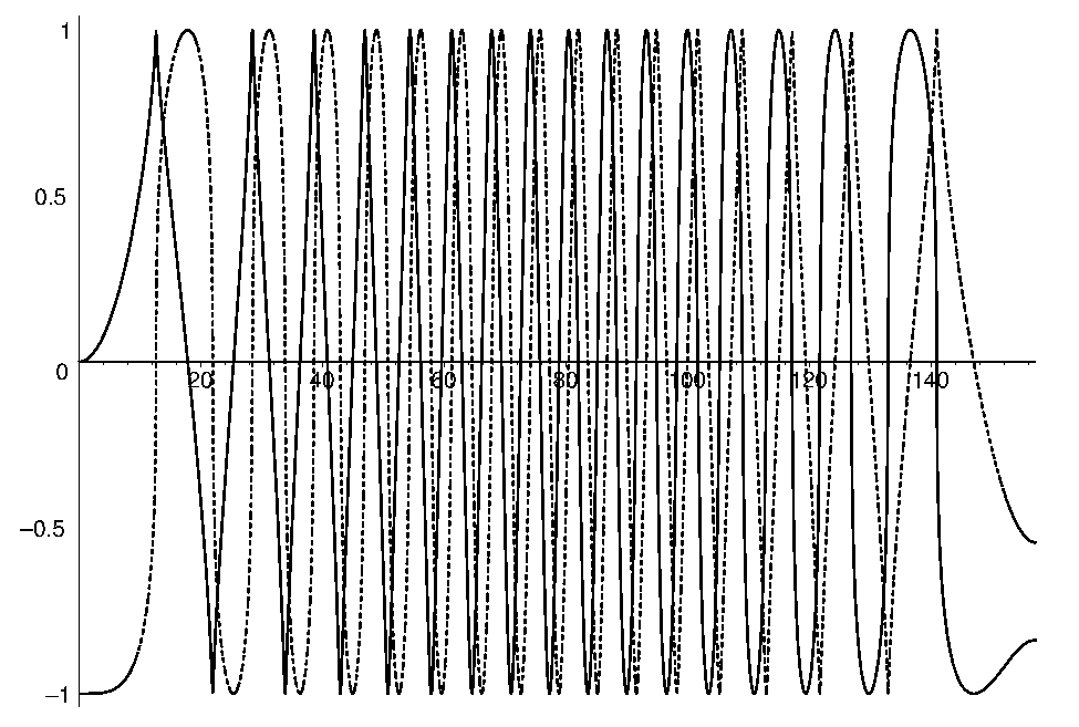
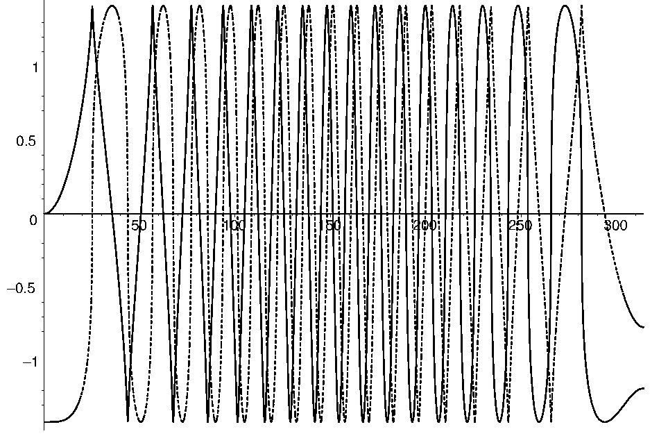
the differential equations (61) and (62) are form invariant with respect to a change in the coupling constant from δ​ω\delta\omega to δ​ω′\delta\omega^{\prime}. This invariance is illustrated in Figures 3 and 4, where typical Bohmian trajectories were computed for both particles. The solutions shown in Figures 3 and 4 were obtained numerically using a 7th-8th-order continuous Runge-Kuta method.

Refer to caption
Figure 3: Bohmian trajectories for two CHO. The trajectories correspond to ω¯=1​fs−1\bar{\omega}=1\,\textrm{fs}^{-1}, δ​ω/ω¯=0.01\delta\omega/\bar{\omega}=0.01, x1​(0)=0x_{1}(0)=0, and x2​(0)=−1x_{2}(0)=-1. The solid line represents the trajectory of x1​(t)x_{1}(t) whereas the dashed line represents that of x2​(t)x_{2}(t). The scale for the ordinates is in Å and the time scale is in fs.
Refer to caption
Figure 4: Bohmian trajectories for two CHO. The trajectories correspond to ω¯=1​fs−1\bar{\omega}=1\,\textrm{fs}^{-1}, δ​ω/ω¯=0.005\delta\omega/\bar{\omega}=0.005, x1​(0)=0x_{1}(0)=0, and x2​(0)=−2x_{2}(0)=-\sqrt{2}. The solid line represents the trajectory of x1​(t)x_{1}(t) whereas the dashed line represents that of x2​(t)x_{2}(t). The scale for the ordinates is in Å and the time scale is in fs. We can observe that the trajectories are identical to the ones shown in the previous Figure, except for the coordinate scales, a result consistent with equations (63)–(65).

It is important to compute, in Bohmian theory, the quantum potential QQ defined as

Q\displaystyle Q =\displaystyle= Q1+Q2\displaystyle Q_{1}+Q_{2}

where

Q1=−ℏ22​m​1P⁡(x1,x2,t)​∂2P⁡(x1,x2,t)∂x12Q_{1}=-\frac{\hbar^{2}}{2m}\frac{1}{\sqrt{P(x_{1},x_{2},t)}}\frac{\partial^{2}\sqrt{P(x_{1},x_{2},t)}}{\partial x_{1}^{2}}

and

Q2=−ℏ22​m​1P⁡(x1,x2,t)​∂2P⁡(x1,x2,t)∂x22.Q_{2}=-\frac{\hbar^{2}}{2m}\frac{1}{\sqrt{P(x_{1},x_{2},t)}}\frac{\partial^{2}\sqrt{P(x_{1},x_{2},t)}}{\partial x_{2}^{2}}.

It is straightforward to compute

Q1\displaystyle Q_{1} =\displaystyle= ℏ​ω¯−12​m​ω¯2​x12\displaystyle\hbar\bar{\omega}-\frac{1}{2}m\bar{\omega}^{2}x_{1}^{2} (66)
+12​ℏ​ω¯​x12​sin2⁡(δ​ω​t)−x22​cos2⁡(δ​ω​t)x12​sin2⁡(δ​ω​t)+x22​cos2⁡(δ​ω​t)\displaystyle+\frac{1}{2}\hbar\bar{\omega}\frac{x_{1}^{2}\sin^{2}\left(\delta\omega t\right)-x_{2}^{2}\cos^{2}\left(\delta\omega t\right)}{x_{1}^{2}\sin^{2}\left(\delta\omega t\right)+x_{2}^{2}\cos^{2}\left(\delta\omega t\right)}
−12​ℏ2m​x22​cos2⁡(δ​ω​t)​sin2⁡(δ​ω​t)(x12​sin2⁡(δ​ω​t)+x22​cos2⁡(δ​ω​t))2,\displaystyle-\frac{1}{2}\frac{\hbar^{2}}{m}\frac{x_{2}^{2}\cos^{2}\left(\delta\omega t\right)\sin^{2}\left(\delta\omega t\right)}{\left(x_{1}^{2}\sin^{2}\left(\delta\omega t\right)+x_{2}^{2}\cos^{2}\left(\delta\omega t\right)\right)^{2}},

and

Q2\displaystyle Q_{2} =\displaystyle= ℏ​ω¯−12​m​ω¯2​x22\displaystyle\hbar\bar{\omega}-\frac{1}{2}m\bar{\omega}^{2}x_{2}^{2} (67)
+12​ℏ​ω¯​x22​cos2⁡(δ​ω​t)−x12​sin2⁡(δ​ω​t)x22​cos2⁡(δ​ω​t)+x12​sin2⁡(δ​ω​t)\displaystyle+\frac{1}{2}\hbar\bar{\omega}\frac{x_{2}^{2}\cos^{2}\left(\delta\omega t\right)-x_{1}^{2}\sin^{2}\left(\delta\omega t\right)}{x_{2}^{2}\cos^{2}\left(\delta\omega t\right)+x_{1}^{2}\sin^{2}\left(\delta\omega t\right)}
−12​ℏ2m​x12​sin2⁡(δ​ω​t)​cos2⁡(δ​ω​t)(x22​cos2⁡(δ​ω​t)+x12​sin2⁡(δ​ω​t))2,\displaystyle-\frac{1}{2}\frac{\hbar^{2}}{m}\frac{x_{1}^{2}\sin^{2}\left(\delta\omega t\right)\cos^{2}\left(\delta\omega t\right)}{\left(x_{2}^{2}\cos^{2}\left(\delta\omega t\right)+x_{1}^{2}\sin^{2}\left(\delta\omega t\right)\right)^{2}},

which yields

Q⁡(x1,x2,t)\displaystyle Q(x_{1},x_{2},t) =\displaystyle= 2​ℏ​ω¯−12​m​ω¯2​(x12+x22)\displaystyle 2\hbar\bar{\omega}-\frac{1}{2}m\bar{\omega}^{2}\left(x_{1}^{2}+x_{2}^{2}\right) (68)
−12​ℏ2m​(x12+x22)​sin2⁡(δ​ω​t)​cos2⁡(δ​ω​t)(x22​cos2⁡(δ​ω​t)+x12​sin2⁡(δ​ω​t))2.\displaystyle-\frac{1}{2}\frac{\hbar^{2}}{m}\frac{\left(x_{1}^{2}+x_{2}^{2}\right)\sin^{2}\left(\delta\omega t\right)\cos^{2}\left(\delta\omega t\right)}{\left(x_{2}^{2}\cos^{2}\left(\delta\omega t\right)+x_{1}^{2}\sin^{2}\left(\delta\omega t\right)\right)^{2}}.

We are now in a position to compute the total bohmian energy for each one of the particles,

E1\displaystyle E_{1} =\displaystyle= K1+V1+Q1\displaystyle K_{1}+V_{1}+Q_{1}
=\displaystyle= ℏ​ω¯+12​ℏ​ω¯​x12​sin2⁡(δ​ω​t)−x22​cos2⁡(δ​ω​t)x12​sin2⁡(δ​ω​t)+x22​cos2⁡(δ​ω​t),\displaystyle\hbar\bar{\omega}+\frac{1}{2}\hbar\bar{\omega}\frac{x_{1}^{2}\sin^{2}\left(\delta\omega t\right)-x_{2}^{2}\cos^{2}\left(\delta\omega t\right)}{x_{1}^{2}\sin^{2}\left(\delta\omega t\right)+x_{2}^{2}\cos^{2}\left(\delta\omega t\right)},
E2\displaystyle E_{2} =\displaystyle= K2+V2+Q2\displaystyle K_{2}+V_{2}+Q_{2}
=\displaystyle= ℏ​ω¯−12​ℏ​ω¯​x12​sin2⁡(δ​ω​t)−x22​cos2⁡(δ​ω​t)x12​sin2⁡(δ​ω​t)+x22​cos2⁡(δ​ω​t),\displaystyle\hbar\bar{\omega}-\frac{1}{2}\hbar\bar{\omega}\frac{x_{1}^{2}\sin^{2}\left(\delta\omega t\right)-x_{2}^{2}\cos^{2}\left(\delta\omega t\right)}{x_{1}^{2}\sin^{2}\left(\delta\omega t\right)+x_{2}^{2}\cos^{2}\left(\delta\omega t\right)},

where Ki=12​m​(d​xid​t)2K_{i}=\frac{1}{2}m\left(\frac{\textrm{d}x_{i}}{\textrm{d}t}\right)^{2} is the kinetic energy of particle ii (obtained from the guidance equations (61) and (62)) and ViV_{i} is the potential for particle ii (neglecting terms in δ​ω/ω¯\delta\omega/\bar{\omega}).

The total energy for the system is just the sum of the individiual energies, yielding

ET=E1+E2=2​ℏ​ω¯,E_{T}=E_{1}+E_{2}=2\hbar\bar{\omega},

the same value as the expected energy of the system.

6 Conclusions and Final Remarks

We see that the expressions obtained for E1E_{1} and E2E_{2} involve an interaction term that makes it impossible to distinguish what part of the energy belongs to the particle x1x_{1} and what part belongs to the particle x2x_{2}, except for some particular values of tt. In the Copenhagen interpretation of QM it does not make any sense to talk about the energy of each oscillator for all tt, as the oscillators are in a quantum superposition and are not in an eigenstate of its hamiltonian operator. In Bohm, it will not make any sense to talk about the energy of each oscillator for all t,t, since the quantum potential creates an interaction between the two oscillators that is of the same order of the other terms in the hamiltonian. Therefore it does not make any sense in the bohmian theory to say that the energy of the photon was transfered to the photodetector (except for very special values of tt).

However, the bohmian interpretation gives an onthological explanation for the indefiniteness of the energy of each particle. Even with the interaction turned off, there is still a quantum nonlocal interaction between the oscillators given by the quantum potential and, in fact, one oscillator is not isolated from the other. This indicates that a real measurement has not yet ocurred. It seems to us that in order for a measurement to take place, a more elaborated description of the photodetection process involving a thermal bath or a macroscopic description must be used. In such case, we expect that the quantum potential will vanish and no further nonlocal interaction will be present after the measurement.

References

  • [1] D. Bohm, Phys. Rev. 85, 166–179 (1952).
  • [2] D. Bohm, Phys. Rev. 85, 180–193 (1952).
  • [3] D. Bohm, Quantum Theory, Dover Publications Inc., New York, 1989.
  • [4] V. Braginsky, F. Ya. Khalili, Quantum Measurement, Cambridge University Press, Cambridge, 1992.
  • [5] C. Cohen-Tannoudji, Processus d´Interaction entre Photons et Atoms, InterEditions et Editions du CNRS, 1988.
  • [6] C. Cohen-Tannoudji, B. Diu, F. Laloe, Quantum Mechanics, Vol. 1, John Wiley and Sons, New York, 1977.
  • [7] J. Acacio de Barros, N. Pinto Neto, “The Causal Interpretation of Quantum Mechanics and the Singularity Problem in Quantum Cosmology”, Nuclear Physics B 57, 247–250 (1997).
  • [8] A. P. French, Vibrations and Waves, W. W. Norton and Co., New York, 1971.
  • [9] H. Goldstein, Classical Mechanics, 2nd Edition, Addison-Wesley Pub. Co., Reading, Massachusetts, 1980.
  • [10] S. W. Groesberg, Advanced Mechanics, John Wiley & Sons, Inc., New York, 1968.
  • [11] P. Holland, The Quantum Theory of Motion, Cambridge University Press, 1993.
  • [12] D. Jackson, Classical Electrodynamics, 2nd Edition, John Wiley & Sons, Inc., New York, 1975.
  • [13] C. Lanczos, The Variational Principles of Mechanics, 4th Edition, Dover Pub. Inc., New York, 1986.
  • [14] L. Mandel and E. Wolf, Optical Coherence and Quantum Optics, Cambridge University Press, 1995.
  • [15] A. Messiah, Quantum Mechanics, Dover Pub. Inc., Mineola, New York, 1999.
  • [16] J. J. Sakurai, Modern Quantum Mechanics, Addison-Wesley Pub. Co., Redwood City, California, 1985.
  • [17] P. Suppes, Representation and Invariance of Scientific Structures, CSLI Publications, Stanford, California, 2002.
  • [18] P. Suppes and J. A. de Barros, “A Random-Walk Approach to Interference”, International Journal of Theoretical Physics, 33(1), 179 (1994).
  • [19] P. Suppes e J. A. de Barros, “Photon Interference with Well Defined Trajectories”, Foundations of Physics Letters 7(6), 501 (1994).
  • [20] P. Suppes, Adonai S. Sant’Anna e J. Acacio de Barros, “A Pure Particle Theory of the Casimir Effect”, Foundations of Physics Letter, 9, 213 (1996).
  • [21] P. Suppes, J.Acacio de Barros, e Adonai S. Sant’Anna, “Violation of Bell’s Inequalities with Local Photons”, Foundations of Physics Letters 9, 551 (1996).
  • [22] K. R. Symon, Mechanics, Third Edition, Addison-Wesley Pub. Co. Inc., Reading, Massachusetts, 1971.