Version August 11, 2026

The topic of entangled imaging has attracted noteworthy attention in recent yearsbib1; bib2; bib3; bib4; bib5; bib7; bib13; bib14. This tecnique exploits the quantum entaglement of the state generated by parametric down-conversion (PDC), in order to retrieve information about an unknown object. In the regime of single photon pair production of PDC, the photons of a pair are spatially separated and propagate through two distinct imaging systems. In the path of one of the photons an object is located. Information about the spatial distribution of the object is not obtained by detection of this photon, but rather by registering the coincidence counts as a function of the other photon position bib1; bib2; bib3; bib4; bib5. In the regime of a large number of photon pairs, this procedure is generalized to the measurement of the signal-idler spatial correlation function of intensity fluctuations bib7. Such a two-arm configuration provides more flexibility in comparison with standard imaging procedures, as e.g. the possibility of illuminating the object with one light frequency and performing a spatially resolved detection in the other arm with a different light frequency, or of processing the information from the object by only operating on the imaging system of arm 2 bib5; bib7. In addition, it opens the possibility of performing coherent imaging by using, in a sense, spatially incoherent light, since each of the two down-converted beams taken separately is described by a thermal-like mixture and only the two-beam state is pure(see e.g. bib5 and bib7).
In this paper we show that it is possible to implement such a scheme using a truly incoherent light, as the radiation produced by a thermal (or quasi-thermal) source. A comparison between thermal and biphoton emission is performed in bib8b, where an underlying duality accompanies the mathematical similarity between the two cases.

Here, we consider a different scheme (Fig.1), appropriate for correlated imaging, in which a thermal beam is divided by a beam-splitter (BS) and the two outgoing beams are handled in the same way as the PDC beams in entangled imaging. A basic analogy between the PDC and the thermal case emerges from our analysis.
Currently there is a debate whether quantum entanglement is necessary to perform correlated imaging bib5; bib13; bib7; bib14. The discussion became very lively after the experiment of bib13 reproduced the results of a ghost image experiment bib3 by using classically correlated beams. We will show here that the spatial correlation of the two beams produced by splitting thermal light, although being completely classical, is enough to qualitatively reproduce all the features of the entangled imaging.

For the sake of comparison we will treat in parallel the cases of entangled beams and of thermal light. For simplicity, we consider only spatial variables and ignore the time argument, which corresponds to using a narrow frequency filter. We will come back to this point in the final part of the paper. In addition, we assume translational invariance in the transverse plane, which amounts to requiring that the cross-section of the source is much larger than the object and all the optical elements. In a future publication we will release these assumptions.

In the entangled case, the signal and idler fields are generated in a type II $\chi^{(2)}$ crystal by a PDC process. Our starting point are the input-output relations of the crystal, which in the plane-wave pump approximation read bib7; bib8; bib9

Here, $b_{i}(\vec{q})=\int\frac{{\rm d}\vec{x}}{2\pi}e^{-\rm i\vec{q}\cdot\vec{x}}b_{i}(\vec{x})$, where $b_{i}(\vec{x})$, are the signal $(i=1)$ and idler $(i=2)$ field envelope operators at the output face of the crystal (distinguished by their orthogonal polarizations), $\vec{x}$ being the position in the transverse plane. $a_{i}\,,\;i=1,2$ are the corresponding fields at the input face of the crystal, and are in the vacuum state. The gain functions $U_{i},V_{i}$ are for example given in bib8.

In the thermal case, we start from the input/output relations of a beam splitter

where $t$ and $r$ are the transmission and reflection coefficients of the mirror, $a$ is a thermal field and $v$ is a vacuum field uncorrelated from $a$. We assume that the thermal state of $a$ is characterized by a Gaussian field statistics, in which any correlation function of arbitrary order is expressed via the second order correlation function bib10:

where $\langle n(\vec{q})\rangle_{th}$ denotes the expectation value of the photon number in mode $\vec{q}$ in the thermal state, and we implicitly used the hypothesis of translational invariance of the source. In particular, the following factorisation property holds bib10:

where $:\,:$ indicates normal ordering. A field with these properties is described by a thermal-like density matrix of the form

where $\left|m,\vec{q}\right\rangle$ denotes the Fock state with $m$ photons in mode $\vec{q}$.
In both the PDC and thermal case, the two outgoing beams travel through two distinct imaging systems, described by their impulse response functions $h_{1}(\vec{x},\vec{x}^{\,\prime})$, $h_{2}(\vec{x},\vec{x}^{\,\prime})$ (see Fig. 1). Arm 1 includes an object. Beam 1 is detected either by a point-like detector $D_{1}$, or by a “bucket” detector, which collects all the light in the detection plane, in any case giving no information on the object spatial distribution. On the other side, detector $D_{2}$ spatially resolves the light fluctuations, as for example an array of pixel detectors. The fields at the detection planes are given by

where $L_{1},L_{2}$ account for possible losses in the imaging systems, and depend on vacuum field operators uncorrelated from $b_{1},b_{2}$. Since they do not contribute to the normally ordered expectation values that we will calculate in the following, their explicit expression is irrelevant. Information about the object is extracted by measuring the spatial correlation function of the intensities detected by $D_{1}$ and $D_{2}$, as a function of the position $\vec{x}_{2}$ of the pixel of $D_{2}$:

All the object information is concentrated in the correlation function of intensity fluctuations:

where $\langle I_{i}(\vec{x}_{i})\rangle=\langle c_{i}^{\dagger}(\vec{x}_{i})c_{i}(\vec{x}_{i})\rangle$ is the mean intensity of the i-th beam. Since $c_{1}$ and $c_{2}^{\dagger}$ commute, all the terms in Eqs. (7),(8) are normally ordered and $L_{1},L_{2}$ can be neglected, thus obtaining

In the thermal case, by taking into account the transformation (2) and that $v$ is in the vacuum state, $b_{1}$ and $b_{2}$ in Eq.(9) can be simply replaced by $ra$ and $ta$. Next, by using Eq.(4), we arrive at the final result

On the other hand, also in the PDC case the four-point correlation function in Eq.(9) has special factorization properties. As it can be obtained from Eq.(1) bib8,

By inserting this result in Eq. (9), one obtains

where, by using relations (1),

There is a clear analogy between the results in the two cases. Apart from the numerical factor $|tr|^{2}$ and the presence of $h_{1}^{*}$ instead of $h_{1}$, the second order correlation $\langle a^{\dagger}(\vec{x})a(\vec{x}^{\,\prime})\rangle$ and the function $\langle n(\vec{q})\rangle_{th}$ play in Eq.(10) the same role as the correlation function $\langle b_{1}(\vec{x})b_{2}(\vec{x}^{\,\prime})\rangle$ and $U_{1}(\vec{q})V_{2}(-q)$ in Eq.(12). Most importantly, in both Eqs.(10)and (12) the modulus is outside the integral, a feature that ensures the possibility of coherent imaging via correlation function (see e.g. bib5). The correlation function $\langle a^{\dagger}(\vec{x})a(\vec{x}^{\,\prime})\rangle$ governs the properties of spatial coherence of the thermal sourcebib10. The correlation length, or transverse coherence length $l_{coh}$, is determined by the inverse of the bandwidth $\Delta q$ of the function $\langle n(\vec{q})\rangle_{th}$. The same holds for the correlation $\langle b_{1}(\vec{x})b_{2}(\vec{x}^{\,\prime})\rangle$, and the function $U_{1}(\vec{q})V_{2}(-\vec{q})$ in the entangled case.

Let us now analyse two paradigmatic examples of imaging systems, mutated from the discussion of bib7, and described in Fig.2.

In both examples the set-up of arm 1 is fixed, and consists of an object, described by a complex transmission function $T(\vec{x})$, and a lens located at a focal distance $f$ from the object and from the detection plane. Hence, $h_{1}(\vec{x}_{1},\vec{x}^{\,\prime}_{1})=-\frac{\rm i}{\lambda f}\exp{\left(-\frac{2\pi\rm i}{\lambda f}\vec{x}_{1}\cdot\vec{x}^{\,\prime}_{1}\right)}T(\vec{x}^{\,\prime}_{1})$, with $\lambda$ being the wavelength. In arm 2 there is a single lens placed at a distance z both from the source and from the detection plane 2.
In the first example we assume z=f (we take the two lenses identical for simplicity), so that $h_{2}(\vec{x}_{2},\vec{x}^{\,\prime}_{2})=-\frac{\rm i}{\lambda f}\exp{\left(-\frac{2\pi\rm i}{\lambda f}\vec{x}_{2}\cdot\vec{x}^{\,\prime}_{2}\right)}\;.$ By inserting these propagators into Eq.(10), and taking into account the expression of $\langle a^{\dagger}(\vec{x})a(\vec{x}^{\,\prime})\rangle$ given by Eq.(3), we obtain

where $\tilde{T}(\vec{q})=\int\frac{\rm d\vec{x}}{2\pi}e^{-\rm i\vec{q}\cdot\vec{x}}T(\vec{x})$ is the amplitude of the diffraction pattern from the object. This has to be compared with the result of the entangled case (see Eq.7 of bib7), where the combination $\vec{x}_{2}+\vec{x}_{1}$ appears instead of $\vec{x}_{2}-\vec{x}_{1}$ and $U_{1}V_{2}$ instead of $\langle n\rangle_{th}$. In both cases, the diffraction pattern from the object can be reconstructed, provided that the spatial bandwidth $\Delta q$ is larger than the maximal $q$ vector appearing in the diffraction pattern, or, equivalently, provided that $l_{coh}<l_{o}$, where $l_{o}$ is the smallest scale of variation of the object spatial distribution. Best performances of the scheme are achieved for spatially incoherent light, $l_{coh}\to 0$. We remind the well-known result that, when $l_{coh}<l_{o}$, no information about the diffraction pattern of the object is obtained by detection of light intensity distribution in arm 1 by an array of pixels.
In the second example, we set z=2f, so that $h_{2}(\vec{x}_{2},\vec{x}^{\,\prime}_{2})=\delta(\vec{x}_{2}+\vec{x}^{\,\prime}_{2})\exp{\left(-\rm i|x_{2}|^{2}\frac{\pi}{\lambda f}\right)}$. Inserting this in Eq. (10), we get:

where in the second line $l_{coh}<l_{o}$ was assumed, so that $\langle n(\vec{q})\rangle_{th}$ is roughly constant in the region of $\vec{q}$ plane where the diffraction pattern does not vanish, and it can be taken out from the integral in (15). In this example the correlation function provides information about the image of the object. A similar result holds for the case of entangled beams (see Eq.(8) of bib7).

Our results appear suprising, if one has in mind the case of a coherent beam impinging on a beam splitter, where the two outgoing fields are uncorrelated, i.e. $G(\vec{x}_{1},\vec{x}_{2})=0$. However, when the input field is an intense thermal beam, i.e. the photon number per mode is not too small, the two outgoing field are well correlated in space. To prove this point, let us consider the number of photons detected in two small identical portions R (“pixels”) of the beams in the near field immediately after the beam splitter, $N_{i}=\int_{R}{\rm d}\vec{x}\,b_{i}^{\dagger}(\vec{x})b_{i}(\vec{x})\>$ $i=1,2$, and the difference $N_{-}=N_{1}-N_{2}$. Making use of the transformation (2), it can be proven that, for $|r|^{2}=|t|^{2}=1/2$, the variance $\langle\delta N_{-}^{2}\rangle=\langle N_{-}^{2}\rangle-\langle N_{-}\rangle^{2}$ is given by

which corresponds exactly to the shot noise level. On the other side, by using the identity $\langle\delta N_{-}^{2}\rangle=\langle\delta N_{1}^{2}\rangle+\langle\delta N_{2}^{2}\rangle-2\langle\delta N_{1}\delta N_{2}\rangle$ and taking into account that $\langle\delta N_{1}^{2}\rangle=\langle\delta N_{2}^{2}\rangle$ for $|r|^{2}=|t|^{2}$, the normalized correlation is given by

For any state $0\leq|C|\leq 1$, where the lower bound corresponds to the coherent state level, and the upper bound is imposed by Cauchy-Schwarz inequality. For the thermal state, provided that the pixel size is not too large with respect to $l_{coh}$, $\langle\delta N_{1}^{2}\rangle\approx\langle N_{1}\rangle+\langle N_{1}\rangle^{2}$, so that the correlation (18) never vanishes. For thermal systems with a large number of photons $\langle N_{1}\rangle/\langle\delta N_{1}^{2}\rangle\approx 1/\langle N_{1}\rangle<<1$, and $C$ can be made close its maximum value. Even more important, it is not difficult to show that Eqs.(17) and (18) hold in any plane linked to the near field plane by a Fresnel transformation, in the absence of losses. In particular, a high level of pixel-by-pixel correlation can be observed in the far-field plane. We remark that, despite $C$ can be made close to 1 by increasing the mean number of photons, the correlation never reaches the quantum level, as shown by Eq.(17).

For the entangled beams produced by PDC, spatial correlation is present both in the near and in the far field, with the ideal result $\langle\delta N_{-}^{2}\rangle=0$, $C=1$ in both planes bib8. In this case, the far field correlation is between symmetric pixels, due to the different way in which the four-point correlation function factorises. In bib7 we analysed the effect of replacing the pure PDC entangled state with two mixtures that exactly preserve the spatial signal-idler quantum correlations, either in the far or in the near field. It turned out that, when considering the “far-field mixture”, the pure state results in the z=f configuration of Fig.2 can be reproduced, but there is no information about the image in the z=2f configuration. The converse is true considering the “near-field mixture”. The two beams generated by splitting thermal light are instead imperfectly correlated both in the near and in the far-field. However, by using intense thermal light, classical intensity correlation is strong enough to reproduce qualitatively the results of both the z=f and the z=2f configuration.
A complete comparison of the performances in the classical and quantum regimes requires extended numerical investigations, describing realistic thermal sources, which is outside the scope of this paper. A key role in this comparison will be played by the issue of the visibility of the information, which is retrieved by subtracting from the measured correlation function (7), the background term $\langle I_{1}(\vec{x}_{1})\rangle\langle I_{2}(\vec{x}_{2})\rangle$ (see Eq.(8)). A measure of the visibility is given by ${\cal V}=\frac{G(\vec{x}_{1},\vec{x}_{2})}{\langle I_{1}(\vec{x}_{1})I_{2}(\vec{x}_{2})\rangle}$.
A first remark concerns the presence of $\langle n(\vec{q})\rangle_{th}$ in Eq. (10) in place of $U_{1}(\vec{q})V_{2}(-q)$ in Eq.(12). As a consequence, in the thermal case $G(\vec{x}_{1},\vec{x}_{2})$ scales as $\langle n(\vec{q})\rangle_{th}^{2}$, while in the entangled case, it scales as $\left|U_{1}(\vec{q})V_{2}(-q)\right|^{2}=\langle n(\vec{q})\rangle+\langle n(\vec{q})\rangle^{2}$, where $\langle n(\vec{q})\rangle=|V_{2}(-\vec{q})|^{2}=|V_{1}(\vec{q})|^{2}$ is the mean number of photons per mode in the PDC beams, and $|U_{1}(\vec{q})|^{2}=1+|V_{1}(\vec{q})|^{2}$ (see e.g bib8). This difference is immaterial when $\langle n(\vec{q})\rangle>>1$, while it becomes relevant for a small photon number, because the background $\langle I_{1}(\vec{x}_{1})\rangle\langle I_{2}(\vec{x}_{2})\rangle\propto\langle n(\vec{q})\rangle^{2}$ is negligible with respect to $G(\vec{x}_{1},\vec{x}_{2})\propto\langle n(\vec{q})\rangle$. Hence, in the regime of single photon pair detection, the entangled case presents a much better visibility of the information with respect to classically correlated thermal beams (see also Klyshko).
A second remark concerns the role of the temporal argument. Calculations that will be reported elsewhere show that the visibility scales as the ratio between the coherence time of the source $\tau_{coh}$ and the detection time (see also bib8b; bib11). In practical applications, this implies that conventional thermal sources, with very small coherence times, are not suitable for the schemes studied here. A suitable source should present a relatively long coherence time, as for example a sodium lamp, or the chaotic light produced by scattering a laser beam through a random medium bib15. As a special example of a thermal source, one can consider the signal field or the idler field generated by PDC. ¹¹ 1 This opens new possibilities, offered by the combination of the correlated imaging from entangled beams and from classically correlated beams.

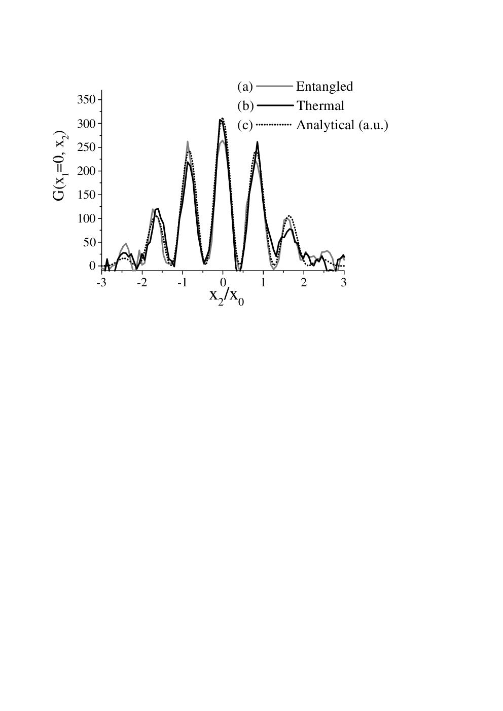
Fig. 3 shows the results of a numerical simulation for the reconstruction of the diffraction pattern of a double slit, in the scheme z=f of Fig.2. It compares the use of signal/idler entangled beams (curve (a)), and two classically correlated beams obtained by symmetrically splitting the idler beam (curve (b)). Parametric gain is such that $\langle n(\vec{q})\rangle\approx 750$ at its maximum for (a), and $\langle n(\vec{q})\rangle\approx 1500$ for (b), so that the the mean photon number of beams $b_{1}$ $b_{2}$ is the same in the two simulations. This example not only shows that in the regime of high photon number the quantum and classical correlation offer similar performances, but also that although the visibility is rather poor, ${\cal V}\approx 0.05$ in both cases, this is enough to correctly retrieve the desired information after a reasonable number of pump shots. The numerical data for the image reconstruction (scheme z=2f of Fig.2) confirm these results.
In conclusion, we have shown a deep analogy between the use of entangled beams and classically correlated beams from a thermal source in imaging schemes based on correlation measurements. As it was already recognized in other contexts (see e.g. Franson), in the small photon number regime, a definite advantage of the quantum configuration is represented by a better visibility.
Our result, that is possible to perform coherent imaging without spatial coherence by using thermal light in combination of a beam splitter is reminiscent of the Hanbury-Brown and Twiss interferometric method for determining the stellar diameterbib16, or of the detection of the fringes arising from interference of two independent thermal sources bib17. However, here, we define a technique to achieve a full coherent imaging with a great deal of flexibility. Since the required correlation is classical, a high quantum efficiency of detectors is not necessary.