Three-mode entanglement by interlinked nonlinear interactions in optical $\chi^{(2)}$ media

The successful demonstration of continuous variable (CV) quantum teleportation furu; bow; zha and dense coding peng opened new perspectives to quantum information technology based on Gaussian states of light. Besides having been recognized as the essential resource for teleportation furu and dense coding ban, the entanglement between two modes of light has been proved as a valuable resource also for cryptography ralph; silb, improvement of optical resolution fabre, spectroscopy spectr, interferometry entdec, state engineering engstat, and tomography of states and operations tomoch; entame.

These achievements stimulated a novel interest in the generation and application of multipartite entanglement jing; zhang; aoki; pvl, which has already received attention in the domain of discrete variables. Multipartite CV entanglement has been proposed to realize cloning at distance (telecloning) telecl0; telecl1, and to improve discrimination of quantum operations gargnano. The separability properties of CV tripartite Gaussian states have been analyzed in geza, where they have been classified into five different classes according to positivity of the three partial transposes that can be constructed. Moreover, it has been pointed out that genuine applications of three-mode entanglement requires fully inseparable tripartite entangled states vlb2000, i.e. states that are inseparable with respect to any grouping of the modes.

Experimental schemes to generate multimode entangled states have been already suggested and demonstrated. The first example, although no specific analysis was made on the entanglement properties (besides verification of teleportation), is provided by the original teleportation experiments of Ref. furu where one party of a twin-beam (TWB) was mixed with a coherent state. A similar scheme, where one party of a TWB is mixed with the vacuum jing has been demonstrated, and applied to controlled dense coding. More recently, a fully inseparable three-mode entangled state has been generated and verified aoki by mixing three independent squeezed vacuum states in a network of beam splitters. In addition, a four-mode entangled state to realize entanglement swapping with pulsed beams have been generated leuch.

All the above schemes are based on parametric sources, either of single-mode squeezing or of two-mode entanglement i.e. TWB, with multipartite entanglement resulting from further interactions in linear optical elements (e.g. beam splitters). In this paper, we focus on a scheme involving a single nonlinear crystal, in which the three-mode entangled state is produced by two type I, non-collinearly phase-matched interlinked bilinear interactions that simultaneously couple the three modes manuscript. A similar interaction scheme, though realized in type II collinear phase-matching conditions, is described in Ref. andrews70. Compared to this work, our choice of non-collinear phase-matching provides remarkable flexibility to our experimental setup, whereas the choice of type I interaction prevents the generation of additional parties. Moreover, we avoid the losses brought about by the mode-matching in multiple beam splitters in that we achieve the three-partite entanglement as soon as we find the configuration that fulfills the phase-matching condition for both interactions.

The paper is structured as follows. In Section II we describe the generation of three-mode entanglement in a single nonlinear crystal where two interlinked bilinear interactions take place simultaneously. We obtain the explicit form in the Fock basis of the outgoing three-mode entangled state, and also address the characterization of entanglement. In Sections III and IV we show how the three-mode entangled state obtained in our scheme, either for initial vacuum state or by seeding the crystal, can be used to build symmetric and asymmetric telecloning machines that achieve optimal fidelity for coherent states. In Section V we show how three-mode entanglement may be used for conditional generation of two-mode entanglement, in particular of TWB state. The scheme is of course less efficient than direct generation of TWB in a parametric amplifier, but it may be of interest in applications where entanglement on-demand is required. In Section VI, we discuss the experimental implementation of our generation scheme. We show the feasibility of experiments in the case of interaction with seeded crystal and report preliminary experimental results. Section VII closes the paper with some concluding remarks.

The interaction Hamiltonian we are going to consider is given by

$H_{int}$ describes two interlinked bilinear interactions taking place among three modes of the radiation field. It can be realized in $\chi^{(2)}$ media by a suitable configuration which will be discussed in Section VI. The effective coupling constants $\gamma_{j}$, $j=1,2$, of the two parametric processes are proportional to the nonlinear susceptibilities and the pump intensities. The Hamiltonian in Eq. (1) has been firstly studied in SmithersLu74, though not for the generation of entanglement. The Hamiltonian admits the following constant of motion

where $N_{j}(t)=\langle a^{\dagger}_{j}(t)a(t)\rangle$ represent the average number of photons in the $j$-th mode. If we take the vacuum $|{\bf 0\rangle}\equiv|0\rangle_{1}\otimes|0\rangle_{2}\otimes|0\rangle_{3}$ as the initial state we have $\Delta=0$ i.e. $N_{1}(t)=N_{2}(t)+N_{3}(t)$ $\forall t$. The expressions for $N_{j}(t)$ can be obtained by the Heisenberg evolution of the field operators, which read as follows

The explicit expressions of the coefficients $f_{j}$, $g_{j}$ and $h_{j}$, $j=1,2,3$, are obtained in appendix A; we omit the time dependence for brevity. By introducing $\Omega=\sqrt{|\gamma_{2}|^{2}-|\gamma_{1}|^{2}}$ we have

The evolved state reads as follows nic

where $U_{t}=\exp\left(-iH_{int}t\right)$ is the evolution operator, and we have already used the conservation law. The state in Eq. (5) is Gaussian, as it can be easily demonstrated by evaluating the characteristic function

where $\lambda_{j}$ are complex numbers, $D_{j}(\lambda_{j})=\exp(\lambda_{j}a^{\dagger}_{j}-\bar{\lambda}_{j}a_{j})$ is a displacement operator for the $j$-th mode, and the primed quantities are obtained by using the Heisenberg evolution of the modes in Eq.s (3). In formulas

Following Ref. geza, the characteristic function can be rewritten as

where ${\bf x}^{T}=(x_{1},x_{2},x_{3},p_{1},p_{2},p_{3})$, $(\cdots)^{T}$ denotes transposition, $\lambda_{j}=2^{-1/2}(p_{j}-ix_{j})$, $j=1,2,3$, and ${\bf C}$ denotes the covariance matrix of the Gaussian state, whose explicit expression can be easily reconstructed from Eq.s (7). The covariance matrix determines the entanglement properties of $|{\bf T}_{0}\rangle$. In fact, since $|{\bf T}_{0}\rangle$ is Gaussian the positivity of the partial transpose is a necessary and sufficient condition for separability geza, which, in turn, is determined by the positivity of the matrices $\Gamma_{j}=\Lambda_{j}{\bf C}\Lambda_{j}-i{\bf J}$ where $\Lambda_{1}=\hbox{Diag}(1,1,1,-1,1,1)$, $\Lambda_{2}=\hbox{Diag}(1,1,1,1,-1,1)$, $\Lambda_{3}=\hbox{Diag}(1,1,1,1,1,-1)$ and ${\bf J}$ is the symplectic block matrix

${\bf I}$ being the $3\times 3$ identity matrix. A numerical evaluation of the eigenvalues of $\Gamma_{j}$ shows that they are nonpositive matrices $\forall j$. Correspondingly, the state in Eq. (5) is fully inseparable i.e. not separable for any grouping of the modes. Notice that the success of a true tripartite quantum protocol, as the telecloning scheme described in the following sections, is a sufficient criterion for the full inseparability of the state $|{\bf T}_{0}\rangle$ vlb2000.

A schematic diagram of our scheme is depicted in Fig. 1. After the preparation of the state $|{\bf T}_{0}\rangle$ a conditional measurement is made on the mode $a_{1}$, which corresponds to the joint measurement of the sum- and difference-quadratures on two modes: mode $a_{1}$ and another reference mode $b$, whose state is to be teleported and cloned. The measurement can be described as the following $\sigma$-dependent POVM acting on the mode $a_{1}$

where $D(\beta)$, $\beta\in{\mathbb{C}}$, is the displacement operator, and $\sigma$ is the preparation of $b$, i.e. the state to be teleported and cloned.

In order to confirm the feasibility of the telecloning scheme presented in the previous section we now show that the same protocol can be implemented also when the state that supports teleportation is generated by Hamiltonian (1) starting from a coherent state in one of the modes, rather than from the vacuum. This may be of interest from the experimental point of view, since seeding a crystal with a coherent beam is a useful technique to align the setup, and allows the verification of the classical evolution of the interacting fields [see Section VI].

The analysis of the scheme is analogue to that of the previous Section, however starting from the initial state $|\alpha,0,0\rangle$ instead of the vacuum. The explicit expression of the evolved state $|{\bf T}_{\alpha}\rangle$ is derived in appendix B. Notice that the conservation law (2) implies that the populations for seeded crystal $N_{j\alpha}=\langle{\bf T}_{\alpha}|a^{\dagger}_{j}a_{j}|{\bf T}_{\alpha}\rangle$ satisfies the relation $N_{1\alpha}-N_{2\alpha}-N_{3\alpha}=|\alpha|^{2}$. We refer the reader to appendix B for the explicit expressions of $N_{j\alpha}$ and for their connections to the populations $N_{j}$ for vacuum input.

A compact expression for the evolved state is the following

where the $f_{j}(t)$, $j=1,2,3$ are given in appendix A. Expression (22) can be easily derived by using the Heisenberg equation of motion for the field-mode $a_{1}(t)$ (see Eq.s (3)). The telecloning process proceed as in the previous Section, with calculations performed using the shifted Fock basis $|\psi_{n}\rangle_{1}\equiv D_{1}(\alpha f_{1})|n\rangle_{1}$, and $|\psi_{n}\rangle_{j}\equiv D_{j}(-\overline{\alpha}\overline{f}_{j})|n\rangle_{j}$, $j=2,3$. If the reference mode $b$ is excited in a pure coherent state $\sigma=|z\rangle\langle z|$, then, as in Section III, the conditional state is pure $\varrho_{\beta}=|\psi_{\beta}\rangle\rangle\langle\langle\psi_{\beta}|$ with

i.e. the product of two independent coherent states. The amplitudes are given by

where the quantities $\kappa_{j}$, $j=2,3$ are given by Eq. (14). The unitary transformation on $a_{2}$ and $a_{3}$ that completes the telecloning is now given by

In fact, the output conditional state coincides with that of Eq. (15), so that the partial traces are identical to those given in Eq. (16). For $N_{2}=N_{3}=N$ we obtain symmetric clones with the same fidelity as in Section III. Moreover conditions (17) and (18) still hold. Notice that also the protocol for asymmetric cloning can be straightforwardly extended to the present seeded scheme.

Another application of the three-mode entangled state of Eq. (5) is the conditional generation of a two-mode entangled state of radiation by on-off photodetection on one of the modes of state $|{\bf T}_{0}\rangle$. Indeed, it is possible to produce a robust two-mode entangled state that approaches a TWB for unit quantum efficiency $\eta$ of the photodetector. In the following we evaluate some properties of the conditional state when $\eta\neq 1$ in order to quantify its closeness to an ideal TWB. Notice that, due to the well known properties of TWB, this scheme also provides a valid check of the whole apparatus from an experimental viewpoint. Let us consider the situation in which a mode of the state $|{\bf T}_{0}\rangle$, say the third mode, is revealed by an on-off photodetector. The probability operator measure (POVM) is two-valued $\{\Pi_{0},\Pi_{1}\}$, $\Pi_{0}+\Pi_{1}={\bf I}$, with the element associated to the ”no photons” result given by

The probability of the outcome is given by

while the conditional output state $\varrho_{0}=\frac{1}{P_{0}}\hbox{Tr}_{3}\left[|{\bf T}_{0}\rangle\langle{\bf T}_{0}|\>\Pi_{0}\right]$ reads as follows

Remind that $N_{1}=N_{2}+N_{3}$. If $\eta=1$ this state reduces to the following TWB

When the efficiency of the detector is not unitary a question arises on how to quantify the closeness of $\varrho_{0}$ to the ideal state $|\psi_{0}\rangle$. From an operational point of view, we can evaluate the photon number correlation between the first and second mode, which is defined as

and is zero in case of TWB. After straightforward calculations we arrive at

which, for any given value of the quantum efficiency $\eta$, is a decreasing function of $N_{2}$ and an increasing function of $N_{3}$. A global quantity to characterize the state in Eq. (27) is the fidelity with a reference TWB state. The natural choice for the reference is the TWB $|\psi_{0}\rangle$, according to the following argument. At first we calculate the fidelity between state (27) and a generic TWB of parameter $\xi$ i.e. $|\xi\rangle=\sqrt{1-\xi^{2}}\sum\xi^{n}|n,n\rangle$, we have

Then, we look for the parameter $\xi$ that maximizes the fidelity. Expression (31) shows that the value of $\xi$ maximizing the fidelity is, independently on $\eta$, $\xi=\sqrt{N_{2}/(1+N_{1})}$. By substituting in Eq. (31) we arrive at

Therefore, the maximum fidelity is obtained for $\eta=1$ and the correct reference state is the TWB $|\psi_{0}\rangle$. In conclusion, the state generated through conditional on/off photodetection on the third mode of $|{\bf T}_{0}\rangle$ is a robust two-mode entangled state with a fidelity to a TWB given by (32). Notice that $\eta<F(\eta)<1$ for any choice of $N_{3}$. The same analysis is valid for a conditional measurement performed on mode $a_{2}$, in which case we obtain an entangled state of modes $a_{1}$ and $a_{3}$ [in this case the role of $N_{2}$ and $N_{3}$ should be exchanged in Eq.s (30), (31), and (32)]. On the other hand, we notice that a conditional photodetection on mode $a_{1}$ does not lead to an entangled state of modes $a_{2}$ and $a_{3}$.

An experimental implementation of the scheme proposed in this paper can be obtained by using a single nonlinear crystal in which the two interactions described by Hamiltonian (1) take place simultaneously. The interactions correspond to two phase-matched second-order nonlinear processes in which five fields interact and two of them do not evolve (parametric approximation). Among the five fields $a_{j}$ involved in the interactions, $a_{4}$ and $a_{5}$ will be the non-evolving pump-fields.

The energy-matching and phase-matching conditions required by the interactions can be written as $\omega_{4}=\omega_{1}+\omega_{3}$, $\omega_{2}=\omega_{3}+\omega_{5}$, $\mathbf{k}_{4}=\mathbf{k}_{1}+\mathbf{k}_{3}$ and $\mathbf{k}_{2}=\mathbf{k}_{3}+\mathbf{k}_{5}$, being $\mathbf{k}_{j}$ the wave-vectors (in the medium) corresponding to $\omega_{j}$, which make angles $\vartheta_{j}$ with the normal to the entrance face of the crystal. It is possible to satisfy these phase-matching conditions with a number of different choices of frequencies and interaction angles depending on the choice of the nonlinear medium. Here we propose an experimental setup based on a $\beta-\rm{BaB}_{2}\rm{O}_{4}$ crystal (BBO, cut angle 32 deg, cross section $10\times 10$ mm² and 4 mm thickness, Fujian Castech Crystals Inc., Fuzhou, China) as the nonlinear medium and the harmonics of a Q-switched amplified Nd:YAG laser (7 ns pulse duration, Quanta-Ray GCR-3-10, Spectra-Physics Inc., Mountain View, CA) as the interacting fields. We choose a compact interaction geometry in which two type I non-collinear interactions with the two pump-beams superimposed in a single beam with mixed polarization take place (see Fig. 3). With reference to Fig. 3, the wavelengths of the interacting modes are $\lambda(\omega_{1})=\lambda(\omega_{3})=1064$ nm, $\lambda(\omega_{4})=\lambda(\omega_{5})=532$ nm and $\lambda(\omega_{2})=355$ nm. The interaction angles, calculated by supposing that the two pump beams propagate along the normal to the crystal entrance face, result to be $\vartheta^{\prime}=37.74$ deg , $\vartheta_{1}=-\vartheta_{3}=10.6$ deg and $\vartheta_{2}=3.5$ deg, and since the crystal we used was cut at 32 deg, it had to be rotated to allow phase matching. In order to demonstrate the feasibility of the scheme in Fig. 3, we adopted the experimental setup depicted in Fig. 4. The fundamental and second harmonic outputs of the Nd:YAG laser were sent to a harmonic separator and then each beam was collimated to a diameter suitable to illuminate the BBO crystal. The polarization of the second harmonic beam emerging from the laser is elliptic, and the two polarization components were separated through a thin-film plate polarizer ($\mathrm{P}_{1}$ in Fig. 4). On the ordinarily polarized component a $\lambda/2$ plate was inserted to modulate the intensity of beam $a_{5}$, without affecting the intensity of the other pump, $a_{4}$. The two beams were then recombined through a second thin-film plate polarizer ($\mathrm{P}_{2}$) and sent to the BBO. As a first verification of the effectiveness of the interaction described by the Hamiltonian (1), we implemented the seeded configuration discussed in Section IV by injecting the BBO with a portion of the fundamental laser output (see Fig. 4) to realize the initial condition for field $a_{1}$.

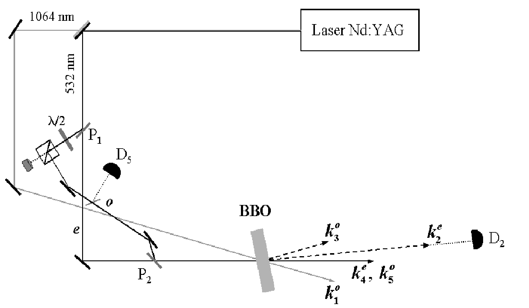
As a first quantitative check, we measured the energy, $\mathrm{E}_{2}$, of the beam generated at $\omega_{2}$ as a function of the energy, $\mathrm{E}_{5}$, of the ordinarily polarized pump-beam for fixed values of the energies of the extraordinarily polarized pump-beam, $\mathrm{E}_{4}$, and of the seed-beam, $\mathrm{E}_{1}$. We preliminarily measured $\mathrm{E}_{1}$ by using a pyroelectric detector (ED200, Gentec Electro-Optics Inc., Quebec, QC, Canada) which also allows checking the stability of the source. By averaging over more than 100 pulses we found a value of about 48 mJ per pulse, only $50\%$ of which is ordinarily polarized, and thus suitable for the interaction. To measure energy $\mathrm{E}_{4}$ we inserted another pyroelectric detector (mod. ED500, Gentec) after $P_{2}$. By averaging again over more than 100 pulses we found a value of about 158 mJ per pulse. To obtain a reliable measurement of $\mathrm{E}_{5}$ we inserted, on the path of beam $a_{5}$, a cube beam splitter and a calibrated glass plate to extract a fraction of the beam. Energy $\mathrm{E}_{5}$ was varied by rotating the $\lambda/2$ plate, and its measurement was performed with the same detector ED500 as before (see $\mathrm{D}_{5}$ in Fig. 4)). To measure the energy $\mathrm{E}_{2}$ of the output pulses we used another pyroelectic detector (PE10, Ophir Optronics Ltd., Jerusalem, Israel, see $\mathrm{D}_{2}$ in Fig. 4)). The values of $\mathrm{E}_{5}$ and $\mathrm{E}_{2}$ were measured simultaneously as averages over the same 20 laser shots at each rotation of the $\lambda/2$ plate. In Fig 5 we show the measured values of $\mathrm{E}_{2}$ (open circles), as a function of the measured values of $\mathrm{E}_{5}$. We can compare the experimental results with the field evolution calculated according to the classical equations manuscript

where $c_{1}=8.3\times 10^{4}(\mathrm{Jm}^{2})^{-1}$ and $c_{2}=2.6\times 10^{5}(\mathrm{Jm}^{2})^{-1}$ are the coupling constants that apply to the present interactions. In Fig 5 we show the values (full circles) of $\mathrm{E}_{2}$ as calculated according to Eq. (33) for the experimental values of $\mathrm{E}_{5}$, and for fixed values $\mathrm{E}_{1}=24$ mJ and $\mathrm{E}_{4}=158$ mJ. The agreement between measured and calculated values is excellent.

We have suggested a scheme to generate fully inseparable three-mode entangled states of radiation based on interlinked bilinear interactions taking place in a single $\chi^{(2)}$ nonlinear crystal. We have shown how the resulting three-mode entanglement can be used to realize symmetric and antisymmetric telecloning machines that achieve optimal fidelity for coherent states. An experimental implementation involving a BBO nonlinear crystal is suggested and the feasibility of the scheme is analyzed. Preliminary experimental results are presented: as a first quantitative check, we measured the energy of the beam generated at $\omega_{2}$ as a function of the energy of the ordinarily polarized pump, for fixed values of the energies of the extraordinarily polarized pump-beam, and of the seed-beam. The agreement between measured and calculated values is excellent.

This work has been supported by the INFM through the project PRA-2002-CLON and by MIUR through the project FIRB-RBAU014CLC. The authors thank M. Cola and N. Piovella (Università di Milano) for fruitful discussions, and F. Paleari and F. Ferri (Università dell’Insubria) for experimental support.

References

- (1) A. Furusawa, J. L. Sørensen, S. L. Braunstein, C. A. Fuchs, H. J. Kimble, and E. S. Polzik, “Unconditional quantum teleportation,” Science 282, 706 (1998).
- (2) W. P. Bowen, N. Treps, B. C. Buchler, R. Schnabel, T. C. Ralph, H. A. Bachor, T. Symul, and P. K. Lau, “Experimental investigation of continuous-variable quantum teleportation,” Phys. Rev. A 67, 032302 (2003).
- (3) T. C. Zhang, K. W. Goh, C. W. Chon, P. Lodahl, and H. J. Kimble , “Quantum teleportation of light beams,” Phys. Rev. A 67, 033802 (2003).
- (4) X. Li, Q. Pan, J. Jing, J. Zhang, C. Xie, and K. Peng, “Quantum dense coding exploiting a bright Einstein-Podolsky-Rosen beam,” Phys. Rev. Lett. 88, 047904 (2002).
- (5) M. Ban, “Quantum dense coding of continuous variables in a noisy quantum channel,” J. Opt. B 2, 786 (2000); T. C. Ralph, E. H. Huntington, “Unconditional continuous-variable dense coding,” Phys. Rev A 66 042321 (2002).
- (6) Ch. Silberhorn, T. C. Ralph, N. Lütkenhaus, and G. Leuchs, “Continuous variable quantum cryptography: beating the 3dB loss limit,” Phys. Rev. Lett. 89, 167901 (2002).
- (7) Ch. Silberhorn, N. Korolkova, and G. Leuchs, “Quantum key distribution with bright entangled beams,” Phys. Rev. Lett. 88, 167902 (2002).
- (8) M. I. Kolobov and C. Fabre, “Quantum limits on optical resolution,” Phys. Rev. Lett. 85 3789 (2000).
- (9) B. E. A. Saleh, B. M. Jost, H.-B. Fei, and M. C. Teich, “Entangled-photon virtual-state spectroscopy,” Phys. Rev. Lett 80 3483 (1998).
- (10) G. M. D’Ariano, M. G. A. Paris and P. Perinotti, “Improving quantum interferometry using entanglement,” Phys. Rev A 65 062106 (2002).
- (11) M. G. A. Paris, M. Cola, and R. Bonifacio, “Quantum state engeneering assisted by entanglement,” Phys. Rev. A 67, 042104 (2003).
- (12) G. M. D’Ariano, and P. Lo Presti, “Quantum tomography for measuring experimentally the matrix elements of an arbitrary quantum operation,” Phys. Rev. Lett. 86 4195 (2001).
- (13) G. M. D’Ariano, P. Lo Presti and M. G. A. Paris, “Using entanglement improves the precision of quantum measurements,” Phys. Rev. Lett. 87, 270404 (2001).
- (14) J. Zhang, C. Xie, and K. Peng, “Controlled dense coding for continuous variables using three-particle entangled states,” Phys. Rev. A 66, 032318 (2002).
- (15) J. Jing, J. Zhang, Y. Yan, F. Zhao, C. Xie, K. Peng, “Experimental demonstration of tripartite entanglement and controlled dense coding for continuous variables,” Phys. Rev. Lett. 90 167903 (2003).
- (16) T. Aoki, N. Takey, H. Yonezawa, K. Wakui, T. Hiraoka, A. Furusawa, and P. van Loock, “Experimental creation of a fully inseparable tripartite continuous-variable state,” Phys. Rev. Lett. 91, 080404 (2003).
- (17) P. van Loock and A. Furusawa, “Detecting genuine multipartite continuous-variable entanglement,” Phys. Rev. A 67, 052315 (2003).
- (18) M. Murao, D. Jonathan, M. B. Plenio, and V. Vedral, “Quantum telecloning and multiparticle entanglement,” Phys. Rev. A 59, 156 (1999);
- (19) P. van Loock, and S. Braunstein, “Telecloning of continuous quantum variables,”Phys. Rev. Lett. 87, 247901 (2001).
- (20) G. M,. D’Ariano, P. Lo Presti, and M. G. A. Paris, “Improved discrimination of unitary transformation by entangled probes,” J. Opt. B, 4, S273 (2002).
- (21) G. Giedke, B. Kraus, M. Lewenstein, and J. I. Cirac, “Separability properties of three-mode Gaussian states,”Phys. Rev. A 64, 052303 (2001).
- (22) P. van Loock, and S. Braunstein, “Multipartite entanglement for continuous variables: a quantum teleportation network,”Phys. Rev. Lett. 84, 3482 (2000).
- (23) O. Glöckl, S. Lorenz, C. Marquardt, J. Heersink, M. Brownnutt, C. Silberhorn, Q. Pan, P. van Loock, N. Korolkova, and G. Leuchs, “Experiment towards continuous-variable entanglement swapping: Highly correlated four-partite quantum state,” Phys. Rev. A 68 012319 (2003).
- (24) A. Allevi, A. Andreoni, M. Bondani, E. Puddu, A. Ferraro, and M. G. A. Paris, “Properties of two interlinked interactions in non-collinear phase-matching,” Optics Lett. 29 (2004), IN PRESS (15 Jan 04, please add the complete reference)
- (25) R. A. Andrews, H. Rabin, and C. L. Tang, “Coupled parametric downconversion and upconversion with simultaneous phase matching,” Phys. Rev. Lett. 25, 605-608 (1970).
- (26) M. E. Smithers, E. Y. C. Lu, “Quantum theory of coupled parametric down-conversion and up-conversion with simultaneous phase matching,” Phys. Rev. A 10, 1874 (1974).
- (27) N. Piovella, M. Cola, and R. Bonifacio, Phys. Rev. A 67, “Quantum fluctuations and entanglement in the collective atomic recoil laser using a Bose-Einstein condensate,” 013817 (2003).
- (28) S.L. Braunstein, V. Buzek, and M. Hillery, “Quantum-information distributors: Quantum network for symmetric and asymmetric cloning in arbitrary dimension and continuous limit,” Phys. Rev. A 63, 052313 (2001); N. J. Cerf, “Asymmetric quantum cloning in any dimension,” J. Mod. Opt. 47, 187 (2000).
- (29) N. J. Cerf, A. Ipe, X. Rottenberg, “Cloning of continuous quantum variables,” Phys. Rev. Lett. 85, 1754 (2000).
- (30) S. L. Braunstein, N. J. Cerf, S. Iblisdir, P. van Loock, and S. Massar, “Optimal cloning of coherent states with a linear amplifier and beam splitters,” Phys. Rev. Lett. 86, 4938 (2001).
- (31) J. Fiurasek, “Optical implemetation of continuous-variables quantum cloning machines,” Phys. Rev. Lett. 86, 4942 (2001).
- (32) N. J. Cerf, S. Iblisdir, and G. van Assche, “Cloning and cryptography with quantum continuous variables,” Eur. Phys. J. D 18, 211 (2002).
Appendix A Heisenberg evolution of modes
In this section we calculate the dynamics generated by the Hamiltonian (1) in the Heisenberg picture. The equations of motion are given by