An All Linear Optical Quantum Memory Based on Quantum Error Correction

Storing qubits for indefinitely long periods of time is a critically important task in quantum information processing. It is needed whenever the quantum teleportation protocols or feed-forward mechanisms are invoked. While photons are ideally suited for the transmission of quantum information, storing them is very difficult. Currently, techniques of mapping quantum information between photons and atomic systems are being developed liu01; phillips01; schori02. Obviously, the simplest quantum memory device for photons can be an optical-fiber loop or a ring cavity. Recently, Pittman and Franson used a Sagnac interferometer to develop a quantum memory device for photons, robust to dephasing pittman02. They concluded that it is, however, the photon loss that typically restricts the storage time.

In this Letter, we present a cyclic quantum memory for photons that can also deal with photon loss. The idea is to use a delay-line loop endowed with a small linear-optical quantum computing (LOQC) circuit knill01; franson02, that runs an error-correction code over and over again on the loop, as depicted in Fig. 1. When multiple error-correcting circuits are placed in series, it allows the transmission of photons over a distance larger than the attenuation length of the fiber. A quantum repeater is a device that executes quantum purification and swapping protocols–with the goal of achieving remote, shared, entanglement briegel98; kok02b; jacobs02. Here, in contrast, we define a “quantum transponder” to be a simple device–one which employs error correction to relay an unknown quantum state with high fidelity down a quantum channel. For quantum key distribution schemes such as BB84 bennett84–only a transponder is required for long-distance key transfer. However, we note that if the fidelity of the transponder is sufficiently high, we can also use it to distribute entanglement by relaying, say, one half of an entangled pair.

Let us first consider our error-correcting code. We use a two-to-four one-error–correcting scheme for protecting the data against photon loss. That is, we encode two qubits into four qubits, such that the resulting code is capable of recovering from the loss of one photon. The encoding is as follows:

This code was first introduced in 1997 by Grassl, Beth and Pellizzari grassl, and it can be implemented using the simple quantum circuit shown in Fig. 2.

The difference between this code, and the usual error-correcting codes based on syndrome detection, is that we do not destroy the ancillæ. In other words, we recover from a single-photon loss without losing any of the four qubits. The error-correction process is shown in Fig. 3, where we assumed that the loss has occurred in the lower-most qubit (the conditional error-correcting operator consisting of a combination of $\sigma_{x}$ and $\sigma_{z}$ acts on the lower-most qubit mode; here, $\sigma_{x}$, $\sigma_{y}$, and $\sigma_{z}$ are the Pauli matrices). Similar circuits work for photon loss in the other three modes.

We can demonstrate how this algorithm works by studying its action on one of the codewords of the code of Eq. (1). For example, consider the codeword $\left|\psi_{0}\right\rangle=\frac{1}{\sqrt{2}}\left(\left|0110\right\rangle+\left|1001\right\rangle\right)$, and suppose that the last qubit is lost (in accordance with Fig. 3). The state of the system is given by the following density operator $\rho_{1}={\textstyle\frac{1}{2}}(\left|011\right\rangle\left\langle 011\right|+\left|100\right\rangle\left\langle 100\right|)$, which is obtained from the initial state $\left|\psi_{0}\right\rangle$ by tracing-out the last qubit. In what follows, it is easier to consider the mixed state $\rho_{1}$ as a probability distribution over the pure states, instead of a density matrix. Thus the mixed state after photon loss can be written as $\rho_{1}=\{(\left|011\right\rangle,{\textstyle\frac{1}{2}}),(\left|100\right\rangle,{\textstyle\frac{1}{2}})\}$.

The quantum nondemolition (QND) device that signals the loss of the last qubit is followed by a qubit state preparation device (photon gun) that substitutes the missing qubit with a new qubit in the ground state $\left|0\right\rangle$. The new density operator is then: $\rho_{2}=\{(\left|0110\right\rangle,{\textstyle\frac{1}{2}}),(\left|1000\right\rangle,{\textstyle\frac{1}{2}})\}$. Including the two ancilla bits, the total system is in the mixed state $\rho_{3}=\rho_{2}\otimes\left|00\right\rangle\left\langle 00\right|=\{(\left|0110\right\rangle\left|00\right\rangle,{\textstyle\frac{1}{2}}),(\left|1000\right\rangle\left|00\right\rangle,{\textstyle\frac{1}{2}})\}$. After applying the Hadamard transform on the ancilla bits, this becomes

The four controlled-$\sigma_{x}$ (CNOT) and controlled-$\sigma_{z}$ (CZ) operations, followed by the the Hadamard transform on the ancilla bits, then yields the mixed state $\rho_{5}=\big\{\big({\textstyle\frac{1}{2}}\big((\left|0110\right\rangle+\left|1001\right\rangle)\left|00\right\rangle+(\left|0110\right\rangle-\left|1001\right\rangle)\left|10\right\rangle\big),{\textstyle\frac{1}{2}}\big),\\ \big({\textstyle\frac{1}{2}}\big((\left|1000\right\rangle+\left|0111\right\rangle)\left|01\right\rangle+(\left|1000\right\rangle-\left|0111\right\rangle)\left|11\right\rangle\big),{\textstyle\frac{1}{2}}\big)\big\}.$

Finally, the measurement outcome of the two ancillæ determines the error-correcting operator on the last qubit. These conditional operators are listed in Table 1. Note that the after the measurement of the ancillæ, the result is always a pure state. Furthermore, all the results are equally likely, so this process does not reveal any information about the original encoded state. It follows immediately from the Table I and Eq. (1) that this will correct the loss of the photon for this particular codeword. In a similar fashion, it can be shown that the error correction will work for an arbitrary input state and a single lost photon.

In the remainder of this paper we will consider optical implementations of this error-correcting code, where the qubits are encoded in two-mode single-photon states. These may either be two spatial modes or two polarization modes knill01; koashi01; franson01; pittman02a.

When we send a photon through an optical fiber of length $d$, the probability of successfully transmitting the photon is given by

Here, the absorption coefficent of the fiber is given by $\alpha$, which is a property of the fiber. The best fibers have an absorbtion length, $1/\alpha$, of about 30 km. We wish to overcome this length restriction with the error correcting codes (ECC) and the linear-optical scheme for implementing two qubit gates that was introduced by Knill, Laflamme, and Milburn (KLM) knill01.

The ECC described above can recover two qubits, given the loss of a single photon. With a perfectly working ECC, the probability of losing zero or one photon in the fiber over a distance $d$ is given by $p_{f}=p^{4}+4p^{3}(1-p)\;,$ where $p$ is given by Eq. (3). Using $p_{f}$ and inverting equation (3) we can calculate an effective absorbtion length for the ECC, or equivalently $\alpha^{\prime}$:

Since our ECC encodes two qubits, we compare $\alpha^{\prime}$ with $2\alpha$, to see if our code is improving the situation or not. Define the function $f(x)$ with $x\equiv\alpha d$, such that

When $x<\ln(3)\approx 1.1$, $f(x)<1$, our ECC (transponder) is increasing the effective absorption length for the qubits we are trying to transmit. So, if we make $d<\ln(3)/\alpha$ the transponder allows us to transmit qubits with higher fidelity than is possible without it. Note that $\lim_{x\rightarrow 0}f(x)=0$, so the absorbtion length can be made arbitrarily large by making $d$ smaller. However, by decreasing $d$ we need to introduce more gates, and the gates introduce errors.

We employ the KLM scheme to implement our quantum circuit. As a consequence, all one-qubit gates can be implemented with minimal errors. Furthermore, we can execute a controlled-not (CNOT) or controlled-sign (CZ) operation efficiently by using ancilla qubits. For $2n$ ancillæ, a CNOT or CZ gate can be successfully executed with probability

assuming all single photon guns, QND measurements, and photon detections work perfectly.

Note that when we send our qubit through a fiber, we are encoding the information in the polarization of a photon, i.e., $|H\rangle\rightarrow|0\rangle\;\;\;|V\rangle\rightarrow|1\rangle\;$. In the “dual-rail” KLM scheme, the qubit is encoded in the path (upper or lower) of the photon. We are therefore sending our qubits in the polarization basis but we are doing error correction in the position basis. This is not a problem because we can use a polarizing beam splitter and appropriate polarization rotators to convert between the two bases. In particular, every KLM-based gate has an equivalent implementation for polarization-encoded qubits.

With imperfect gates, our equation for $r\equiv\alpha^{\prime}/2\alpha$ becomes

where $p_{t}$ is the probability that all the gates in the quantum transponder work correctly. We can see that for $p_{t}<1$, the minimum of $r$ is no longer at $x=0$ (where the transponder stations are placed back-to-back), since the second term is infinite at that point. Figure 4 is a contour plot of Eq. (7) as a function of $x$ and $p_{t}$. Note that the losses from the gates that do the encoding and decoding of the qubits are one-time losses, and become relatively unimportant for long transmission lines.

Using Eq. (6), and noting that there are four CNOT and four CZ gates in each transponder, we can write $p_{t}=[n/(n+1)]^{16}$. The value of $n$ for which the minimum drops below one is at $n=56$. So we need at least 112 ancilla qubits at each gate for the transponder to transmit qubits more reliably than the fiber without error correction.

Let us now consider the probability of success for a single quantum transponder with inefficient detectors. Suppose, as in Fig. 3, we use the QND device proposed by Kok et al. kok02. This device operates by teleporting the input photon to the output mode, using coincidence counting in a CNOT-operated Bell measurement. The photon loss is then signalled by finding a single detector click. In this case, there is always a photon in the output mode, and we do not need the four single-photon guns.

As shown in Fig. 3, the transponder consists of two single-photon guns (SPG), four QND devices, six one-qubit gates, four CNOT gates, four CZ gates, and two photodetectors (see the first row in Table 2). The single-photon QND measurement can be accomplished with two SPGs, two CNOT gates, two Hadamard gates, and two photodetectors. The first Hadamard and CNOT gates are for Bell state preparation, and the Bell state measurement can be made by CNOT and Hadamard and measurements in the computational basis. For each CNOT gate, we have two one-qubit gates and a CZ gate.

Given that we use $2n$ ancilla photons for each CZ gate, we need to have $2n$ SPGs and $2(n+1)$ photodetectors. Altogether, we need to have 38 one-qubit gates, sixteen CZ gates, $10+32n$ SPGs, and $10+32(n+1)$ photo detectors. Hence the probability of success for the transponder is given by $p_{t}=p_{\rm one}^{38}~p_{\rm two}^{16}~p_{\rm spg}^{10+32n}~\eta^{10+32n}\;,$ where $p_{\rm one}$, $p_{\rm two}$, and $p_{\rm spg}$ are the success probability of the QND measurement, the one-qubit gate, the two-qubit (CZ) gate, and a SPG, respectively. Note that $\eta$ denotes the quantum efficiency of the photo detector, where $10+32n$ detectors among $10+32(n+1)$ should click for perfect gate operations.

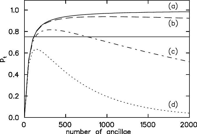
Now let us assume that the number of ancilla photons used for a two-qubit gate is $2n$, which gives $p_{\rm two}=n^{2}/(n+1)^{2}$. Hence, the number of ancilla photons may be optimized for a given quantum efficiency of the photodetectors and the success probability of the single photon guns. Let us assume for now that $p_{\rm one}=p_{\rm spg}=1$. Then $p_{t}$ is given by

For example, if $1-\eta=10^{-5}$, taking $n=16$ yields $p_{t}\approx 0.14$. With $n=160$ we have $p_{t}\approx 0.78$. A typical value that the success probability needs to beat is 0.75. In Fig. 5 we plot $p_{t}$ as a function of the number of ancillæ with different detector efficiencies $\eta$.

In conclusion, we have presented an error-correction scheme that encodes an unknown two photon state into four photons, up to one of which can be lost in the transmission. This device acts as a simple repeater or quantum transponder when it is placed in series, and it acts as an optical quantum memory when it is inserted in an optical loop. Since the absorbtion length for two photons in a fiber is $1/(2\alpha)$, the storage time is given by $T_{f}=1/(2\alpha\nu)$ where $\nu$ is the speed of light in the fiber. With error correction we can increase the storage time to $T_{f}/r$. We gave a quantitative analysis of the behaviour of this quantum memory in several situations, deriving values for the optimal length of the loop, and characterizing the performance in the presence of detector losses.

Using this scheme, the conversion between flying qubits and stationary qubits in memory is not necessary with LOQC, as the memory and quantum logic gates are composed of the same optical resources. The delay line, when rolled out, is a fiber quantum communication line with simple LOQC transponders, suitable for the BB84 quantum key distribution protocol bennett84.

This work was carried out at the Jet Propulsion Laboratory, California Institute of Technology, under a contract with the National Aeronautics and Space Administration. We wish to thank J.D. Franson, G.J. Milburn, and T.B. Pittman for stimulating discussions, and we would like to acknowledge support from the National Security Agency, the Advanced Research and Development Activity, the Defense Advanced Research Projects Agency, the National Reconnaissance Office, and the Office of Naval Research. R.M.G. and P.K. thank the National Research Council and NASA Code Y for support.

References

- (1) C. Liu, Z. Dutton, C.H. Behroozi, and L.V. Hau, Nature 409, 490 (2001).
- (2) D.F. Phillps, A. Fleischhauer, A. Mair, and M.D. Lukin, Phys. Rev. Lett. 86, 783 (2001).
- (3) C. Schori, B. Julsgaard, J.L. Sørensen, and E.S. Polzik, Phys. Rev. Lett. 89, 057903 (2002).
- (4) T.B. Pittman and J.D. Franson, Phys. Rev. A 66, 062302 (2002).
- (5) E. Knill, R. Laflamme, and G.J. Milburn, Nature, 409, 46 (2001).
- (6) J.D. Franson, M.M. Donegan, M.J. Fitch, B.C. Jacobs, and T.B. Pittman, Phys. Rev. Lett. 89, 137901 (2002).
- (7) H.-J. Briegel, W. Dür, J.I. Cirac, and P. Zoller, Phys. Rev. Lett. 81, 5932 (1998).
- (8) P. Kok, C.P. Williams, and J.P. Dowling, “Practical quantum repeaters with linear optics and double-photon guns,” quant-ph/0203134.
- (9) B.C. Jacobs, T.B. Pittman, and J.D. Franson, Phys. Rev. A 66, 052307 (2002).
- (10) C.H. Bennett and G. Brassard, Proceedings of the IEEE International Conference on Computers, Systems, and Signal Processing, 175 (IEEE, New York, NY, 1984).
- (11) M. Grassl, T. Beth, and T. Pellizzari, Phys. Rev. A 56, 33 (1997).
- (12) M. Koashi, T. Yamamoto, and N. Imoto, Phys. Rev. A 63, 030301 (2001).
- (13) T.B. Pittman, B.C. Jacobs, and J.D. Franson, Phys. Rev. A 64, 062311 (2001).
- (14) T.B. Pittman, B.C. Jacobs, and J.D. Franson, Phys. Rev. Lett. 88, 257902 (2002).
- (15) P. Kok, H. Lee, and J.P. Dowling, Phys. Rev. A 66, 063814 (2002).