Scalability of Shor’s algorithm with a limited set of rotation gates

Shor’s algorithm factors an integer $N=N_{1}N_{2}$ by finding the period $r$ of a function $f(k)=m^{k}\bmod N$ where $1<m<N$ and ${\rm gcd}(m,N)=1$. Provided $r$ is even and $f(r/2)\neq N-1$ the factors are $N_{1}={\rm gcd}(f(r/2)+1,N)$ and $N_{2}={\rm gcd}(f(r/2)-1,N)$, where ${\rm gcd}$ denotes the greatest common divisor. The probability of finding a suitable $r$ given a randomly selected $m$ such that ${\rm gcd}(m,N)=1$ is greater than $0.75$ Nielson and Chuang 2000. Thus on average very few values of $m$ need to be tested to factor $N$.

The quantum heart of Shor’s algorithm can be viewed as a subroutine that generates numbers of the form $j\simeq c2^{2L}/r$. To distinguish this from the necessary classical pre-and postprocessing, this subroutine will be referred to as QPF (quantum period finding). For physical reasons, the probability $s$ that QPF will successfully generate useful data may be quite low with many repetitions required to work out the period $r$ of a given $f(k)=m^{k}\bmod N$. Using this terminology, Shor’s algorithm consists of classical preprocessing, potentially many repetitions of QPF with classical postprocessing and possibly a small number of repetitions of this entire cycle. This cycle is summarized in Fig 1.

A number of different quantum circuits implementing QPF have been designed Vedral et al. 1996; Gossett 1998; Beauregard 2003; Zalka 1998. Table 1 summarizes the number of qubits required and the depth of each of these circuits. The depth of a circuit has been defined to be the minimum number of 2-qubit gates that must be applied sequentially to complete the circuit. It has been assumed that multiple disjoint 2-qubit gates can be implemented in parallel, hence the total number of 2-qubit gates can be significantly greater that the depth. For example, the Beauregard circuit has a 2-qubit gate count of $8L^{4}$ to first order in $L$.

Note that in general the depth of the circuit can be reduced at the cost of additional qubits.

The underlying algorithm common to each circuit begins by initializing the quantum computer to a single pure state $|0\rangle_{2L}|0\rangle_{L}$. Note that for clarity the computer state has been broken into a $2L$-qubit $k$-register and an $L$-qubit $f$-register. The meaning of this will become clearer below.

Step two is to Hadamard transform each qubit in the $k$-register yielding

Step three is to calculate and store the corresponding values of $f(k)$ in the $f$-register

Note that this step requires additional ancilla qubits. The exact number depends heavily on the circuit used.

Step four can actually be omitted but it explicitly shows the origin of the period $r$ being sought. Measuring the $f$-register yields

where $k_{0}$ is the smallest value of $k$ such that $f(k)$ equals the measured value $f_{M}$.

Step five is to apply the quantum Fourier transform

to the $k$-register resulting in

The probability of measuring a given value of $j$ is thus

If $r$ divides $2^{2L}$ Eq (6) can be evaluated exactly. In this case the probability of observing $j=c2^{2L}/r$ for some integer $0\leq c<r$ is $1/r$ whereas if $j\neq c2^{2L}/r$ the probability is 0. This situation is illustrated in Fig 2(a). However if $r$ divides $2^{2L}$ exactly a quantum computer is not needed as $r$ would then be a power of 2 and easily calculable. When $r$ is not a power of 2 the perfect peaks of Fig 2(a) become slightly broader as shown in Fig 2(b). All one can then say is that with high probability the value $j$ measured will satisfy $j\simeq c2^{2L}/r$ for some $0\leq c<r$.

Given a measurement $j\simeq c2^{2L}/r$ with $c\neq 0$, classical postprocessing is required to extract information about $r$. The process begins with a continued fraction expansion. To illustrate, consider factoring 143 ($L=8$). Suppose we choose $m$ equal 2 and the output $j$ of QPF is 31674. The relation $j\simeq c2^{2L}/r$ becomes $31674\simeq c65536/r$. The continued fraction expansion of $c/r$ is

The continued fraction expansion of any number between 0 and 1 is completely specified by the list of denominators which in this case is $\{2,14,2,10,52\}$. The $n$th convergent of a continued fraction expansion is the proper fraction equivalent to the first $n$ elements of this list. An introductory exposition and further properties of continued fractions are described in Ref Nielson and Chuang 2000.

The period $r$ can be sought by substituting each denominator into the function $f(k)=2^{k}\bmod 143$. With high probability only the largest denominator less than $2^{L}$ will be of interest. In this case $2^{60}\bmod 143=1$ and hence $r=60$.

Two modifications to the above are required. Firstly, if $c$ and $r$ have common factors, none of the denominators will be the period but rather one will be a divisor of $r$. After repeating QPF a number of times, let $\{j_{m}\}$ denote the set of measured values. Let $\{c_{mn}/d_{mn}\}$ denote the set of convergents associated with each measured value $\{j_{m}\}$. If a pair $c_{mn}$, $c_{m^{\prime}n^{\prime}}$ exists such that ${\rm gcd}(c_{mn},c_{m^{\prime}n^{\prime}})=1$ and $d_{mn}$, $d_{m^{\prime}n^{\prime}}$ are divisors of $r$ then $r={\rm lcm}(d_{mn},d_{m^{\prime}n^{\prime}})$, where ${\rm lcm}$ denotes the least common multiple. It can be shown that given any two divisors $d_{mn}$, $d_{m^{\prime}n^{\prime}}$ with corresponding $c_{mn}$, $c_{m^{\prime}n^{\prime}}$ the probability that ${\rm gcd}(c_{mn},c_{m^{\prime}n^{\prime}})=1$ is at least $1/4$ Nielson and Chuang 2000. Thus only $O(1)$ different divisors are required. In practice, it will not be known which denominators are divisors so every pair $d_{mn}$, $d_{m^{\prime}n^{\prime}}$ with ${\rm gcd}(c_{mn},c_{m^{\prime}n^{\prime}})=1$ must be tested.

The second modification is simply allowing for the output $j$ of QPF being useless. Let $s$ denote the probability that $j=\lfloor c2^{2L}/r\rfloor$ or $\lceil c2^{2L}/r\rceil$ for some $0<c<r$ where $\lfloor\rfloor$, $\lceil\rceil$ denote rounding down and up respectively. Such values of $j$ will be called useful as the denominators of the associated convergents are guaranteed to include a divisor of $r$. The period $r$ sought can always be found provided $O(1/s)$ runs of QFT can be performed.

To summarize, as each new value $j_{m}$ is measured, the denominators $d_{mn}$ less than $2^{L}$ of the convergents of the continued fraction expansion of $j_{m}/2^{2L}$ are substituted into $f(k)=m^{k}\bmod N$ to determine whether any $f(d_{mn})=1$ which would imply that $r=d_{mn}$. If not, every pair $d_{mn}$, $d_{m^{\prime}n^{\prime}}$ with associated numerators $c_{mn}$, $c_{m^{\prime}n^{\prime}}$ satisfying ${\rm gcd}(c_{mn},c_{m^{\prime}n^{\prime}})=1$ must be tested to see whether $r={\rm lcm}(d_{mn},d_{m^{\prime}n^{\prime}})$. Note that as shown in Fig 1, if $r$ is even or $m^{r/2}\bmod N=\pm 1\bmod N$ then the entire process needs to be repeated $O(1)$ times. Thus Shor’s algorithm always succeeds provided $O(1/s)$ runs of QFT can be performed.

A circuit that implements the QFT of Eq (4) is shown in Fig 3(a). Note the use of controlled rotations of magnitude $\pi/2^{d}$. In matrix notation these 2-qubit operations correspond to

The approximate QFT (AQFT) circuit is very similar with just the deletion of rotation gates with $d$ greater than some $d_{\rm max}$. For example, Fig 3(b) shows an AQFT with $d_{\rm max}=1$. Let $[j]_{m}$ denote the $m$th bit of $j$. The AQFT equivalent to Eq (4) is Coppersmith 1994

where $\tilde{\sum}_{mn}$ denotes a sum over all $m$, $n$ such that $0\leq m,n<2L$ and $2L-d_{\rm max}+1\leq m+n<2L$. It has been shown by Coppersmith that the AQFT is a good approximation of the QFT Coppersmith 1994 in the sense that the phase of individual computational basis states in the output of the AQFT differ in angle from those in the output of the QFT by at most $2\pi L2^{-d_{\rm max}}$. The purpose of this paper is to investigate in detail the effect of using the AQFT in Shor’s algorithm.

When the 7-qubit Steane code Steane 1996; Calderbank and Shor. 1995; Nielson and Chuang 2000 and its concatenated generalizations are used to do computation, only the limited set of gates cnot, Hadamard ($H$), $X$, $Z$, $S$ and $S^{{\dagger}}$ can be implemented easily, where

Complicated circuits of depth in the hundreds and requiring a minimum of 22 qubits are required to implement the $T$ and $T^{{\dagger}}$ gates Nielson and Chuang 2000

Note however that if it is acceptable to add an additional 15 qubits for every $T$ and $T^{{\dagger}}$ gate in a sequence of fault-tolerant single-qubit gates (see for example Eq (13)), the effective depth of each $T$ and $T^{{\dagger}}$ gate circuit can be reduced to 2. Together, the set cnot, $H$, $X$, $Z$, $S$, $S^{{\dagger}}$, $T$ and $T^{{\dagger}}$ enables the implementation of arbitrary 1- and 2-qubit gates via the Solovay-Kitaev theorem Kitaev 1997; Nielson and Chuang 2000. For example, the controlled $\pi/2^{d}$ gate can be decomposed into a single cnot and three single-qubit rotations as shown in Fig 4.

Approximating single-qubit $\pi/2^{d}$ rotations using the fault-tolerant gate set is much more difficult. For convenience, such rotations will henceforth be denoted by $R_{2^{d}}$. The simplest (least number of fault-tolerant gates) approximation of the $R_{128}$ single-qubit rotation gate that is more accurate than simply the identity matrix is the 31 gate product

Eq (13) was determined via an exhaustive search minimizing the metric

The rationale of Eq (14) is that if $U$ and $V$ are similar, $U^{{\dagger}}V$ will be close to the identity matrix (possibly up to some global phase) and the absolute value of the trace will be close to 2. By subtracting this absolute value from 2 and dividing by 2 a number between 0 and 1 is obtained. The overall square root is required to ensure that the triangle inequality

is satisfied.

The identity matrix is a good approximation of $R_{128}$ in the sense that ${\rm dist}(R_{128},I)=8.7\times 10^{-3}$. Eq (13) is only slightly better with ${\rm dist}(R_{128},U_{31})=8.1\times 10^{-3}$. A 46 gate sequence has been found satisfying ${\rm dist}(R_{128},U_{46})=7.5\times 10^{-4}$. Note that this is still only 10 times better than doing nothing. Further investigation of the properties of fault-tolerant approximations of arbitrary single-qubit unitaries will be performed in the near future. For the present discussion it suffices to know that the number of gates grows somewhere between linearly and quadratically with $\ln(1/{\delta})$ Nielson and Chuang 2000 where $\delta={\rm dist}(R,U)$, $R$ is the rotation being approximated, and $U$ is the approximating product of fault-tolerant gates (the exact scaling is not known). In particular, this means that approximating a rotation gate $R_{2^{d}}$ with accuracy $\delta=1/2^{d}$ requires a number of gates that grows linearly or quadratically with $d$.

In addition to the inconveniently large number of fault-tolerant gates $n_{\delta}$ required to achieve a given approximation $\delta$, each individual gate in the approximating sequence must be implemented with probability of error $p$ less than $O(\delta/n_{\delta})$. Note that $\delta$ is not a probability of error but rather a measure of the distance between the ideal gate and the approximating product so this relationship is not exact. If the required probability $p\sim\delta/n_{\delta}=1/(n_{\delta}2^{d})$ is too small to be achieved using a single level of QEC, the technique of concatenated QEC must be used. Roughly speaking, if a given gate can be implemented with probability of error $p$, adding an additional level of concatenation Knill et al. 1996 leads to an error rate of $cp^{2}$ where $c<1/p$. If the Steane code is used with seven qubits for the code and an additional five qubits for fault-tolerant correction, every additional level of concatenation requires 12 times as many qubits. This implies that if a gate is to be implemented with accuracy $1/(n_{\delta}2^{d})$, the number of qubits $q$ scales as $O(d^{\ln_{2}12})=O(d^{3.58})$. While this is a polynomial number of qubits, for even moderate values of $d$ this leads to thousands of qubits being used to achieve the required gate accuracy.

Given the complexity of implementing $T$ and $T^{{\dagger}}$ gates, the number of fault-tolerant gates required to achieve good approximations of arbitrary rotation gates and the large number of qubits required to achieve sufficiently reliable operation, it is clear that for practical reasons the use of $\pi/2^{d}$ rotations must be restricted to those with very small $d$.

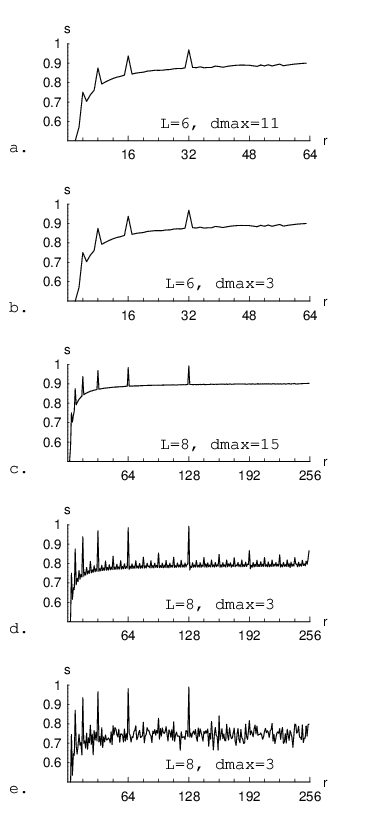
Different values of $r$ (the period of $f(k)=x^{k}\bmod N$) imply different probabilities $s$ that the value $j$ measured at the end of QPF will be useful (see Fig 1). In particular, as discussed in Section I if $r$ is a power of 2 the probability of useful output is much higher (see Fig 2). This section investigates how sensitive $s$ is to variations in $r$. Recall Eq (6) for the probability of measuring a given value of $j$. When the AQFT (Eq (10) is used this becomes

The probability $s$ of useful output is thus

where $\{{\rm useful}~j\}$ denotes all $j=\lfloor c2^{2L}/r\rfloor$ or $\lceil c2^{2L}/r\rceil$ such that $0<c<r$. Fig 5 shows $s$ for $r$ ranging from 2 to $2^{L}-1$ and for various values of $L$ and $d_{\rm max}$. The decrease in $s$ for small values of $r$ is more a result of the definition of $\{{\rm useful}~j\}$ than an indication of poor data. When $r$ is small there are few useful values of $j\simeq c2^{2L}/r\rceil$, $0<c<r$ and a large range states likely to be observed around each one resulting superficially in a low probability of useful output $s$ as $s$ is the sum of the probabilities of observing only values $j=\lfloor c2^{2L}/r\rfloor$ or $\lceil c2^{2L}/r\rceil$, $0<c<r$. However, in practice values much further from $j\simeq c2^{2L}/r$ can be used to obtain useful output. For example if $r=4$ and $j=16400$ the correct output value (4) can still be determined from the continued fraction expansion of $16400/65536$ which is far from the ideal case of $16384/65536$. To simplify subsequent analysis each pair $(L,d_{\rm max})$ will from now on be associated with $s(2^{L-1}+2,L,d_{\rm max})$ which corresponds to the minimum value of $s$ to the right of the central peak. The choice of this point as a meaningful characterization of the entire graph is justified by the discussion above.

For completeness, Fig 5(e) shows the case of noisy controlled rotation gates of the form

where $\delta$ is a normally distributed random variable of standard deviation $\sigma$. This has been included to simulate the effect of using approximate rotation gates built out of a finite number of fault-tolerant gates. The general form and probability of successful output can be seen to be similar despite $\sigma=\pi/32$. This $\sigma$ corresponds to $\pi/2^{d_{\rm max}+2}$. For a controlled $\pi/64$ rotation, single-qubit rotations of angle $\pi/128$ are required, as shown in Fig 4. Fig 5(e) implies that it is acceptable for this rotation to be implemented within $\pi/512$, implying

is an acceptable approximation of $R_{128}$. Given that ${\rm dist}(R_{128},U)=2.1\times 10^{-3}$, the 46 fault-tolerant gate approximation of $R_{128}$ mentioned above is adequate.

In order to determine how the probability of useful output $s$ depends on both the integer length $L$ and the minimum allowed controlled rotation $\pi/2^{d_{\rm max}}$, Eq (17) was solved with $r=2^{L-1}+2$ as discussed in Section IV. Fig 6 contains semilog plots of $s$ versus $L$ for different values of $d_{\rm max}$. Note that Eq (17) grows exponentially more difficult to solve as $L$ increases.

For $d_{\rm max}$ from 0 to 5, the exponential decrease of $s$ with increasing $L$ is clear. Asymptotic lines of best fit of the form

have been shown. Note that for $d_{\rm max}>0$, the value of $t$ increases by greater than a factor of 4 when $d_{\rm max}$ increases by 1. This enables one to generalize Eq (20) to an asymptotic lower bound valid for all $d_{\rm max}>0$

with the constant of proportionality approximately equal to 1.

Keeping in mind that the required number of repetitions of QPF is $O(1/s)$, one can relate $L_{\rm max}$ to $d_{\rm max}$ by introducing an additional parameter $f_{\rm max}$ characterizing the acceptable number of repetitions of QPF

Available RSA Rivest et al. 1978 encryption programs such as PGP typically use integers of length $L$ up to 4096. The circuit in Vedral et al. 1996 runs in $150L^{3}$ steps when an architecture that can interact arbitrary pairs of qubits in parallel is assumed and fault-tolerant gates are used. Note that to first order in $L$ the number of steps does not increase as additional levels of QEC are used. Thus $\sim$$10^{13}$ steps are required to perform a single run of QPF. On an electron spin or charge quantum computer Burkard et al. 2000; Hollenberg et al. 2003 running at 10GHz this corresponds to $\sim$$15$ minutes of computing. If we assume $\sim$24 hours of computing is acceptable then $f_{\rm max}\sim 10^{2}$. Substituting these values of $L_{\rm max}$ and $f_{\rm max}$ into Eq (22) gives $d_{\rm max}=6$ after rounding up. Thus provided controlled $\pi/64$ rotations can be implemented accurately, implying the need to accurately implement $\pi/128$ single-qubit rotations, it is conceivable that a quantum computer could one day be used to break a 4096-bit RSA encryption in a single day.

We have demonstrated the robustness of Shor’s algorithm when a limited set of rotation gates is used. The length $L_{\rm max}$ of the longest factorable integer can be related to the maximum acceptable runs of quantum period finding $f_{\rm max}$ and the smallest accurately implementable controlled rotation gate $\pi/2^{d_{\rm max}}$ via $L_{\rm max}\sim 4^{d_{\rm max}-1}\log_{2}f_{\rm max}$. Integers thousands of digits in length can be factored provided controlled $\pi/64$ rotations can be implemented with rotation angle accurate to $\pi/256$. Sufficiently accurate fault-tolerant constructions of such controlled rotation gates have been described.

References

- Shor (1994) P. W. Shor, Proceedings. 35th Annual Symposium on Foundations of Computer Science pp. 124–134 (1994).
- Shor (2000) P. W. Shor, quant-ph/0005003 (2000).
- Coppersmith (1994) D. Coppersmith, IBM Research Report p. RC19642 (1994).
- Nielson and Chuang (2000) M. A. Nielson and I. L. Chuang, Quantum Computation and Quantum Information (Cambridge University Press, Cambridge, 2000).
- Vedral et al. (1996) V. Vedral et al., Phys. Rev. A 54, 147 (1996).
- Gossett (1998) P. Gossett, quant-ph/9808061 (1998).
- Beauregard (2003) S. Beauregard, Quantum Inform. Compu. 3, 175 (2003).
- Zalka (1998) C. Zalka, quant-ph/9806084 (1998).
- Steane (1996) A. M. Steane, Proc. R. Soc. London A 425, 2551 (1996).
- Calderbank and Shor. (1995) A. R. Calderbank and P. W. Shor., Phys. Rev. A 54, 1098 (1995).
- Kitaev (1997) A. Y. Kitaev, Russ. Math. Surv. 52, 1191 (1997).
- Knill et al. (1996) E. Knill et al., quant-ph/9610011 (1996).
- Rivest et al. (1978) R. L. Rivest et al., Communications of the ACM 21, 120 (1978).
- Burkard et al. (2000) G. Burkard et al., Fortschr. Physik 48, 965 (2000).
- Hollenberg et al. (2003) L. C. L. Hollenberg et al., cond-mat/0306235 (2003).