Mapping the Wigner distribution function of the Morse oscillator into a semi-classical distribution function Preprint:  IFT-P.013/03 April 2003

The Wigner description in phase-space [1] provides a tool for comparing quantum and classical dynamics [2]. In a previous paper [3] we introduced a mapping relating the Wigner distribution function (WDF) corresponding to a given wave function, solution of the Schrödinger equation to a semiclassical distribution function (SDF) satisfying the classical Liouville equation with the same potential. So far this mapping was applied to the ground state of the square well [3], the Pöschl-Teller potential [4] and to a modified harmonic oscillator potential [4].

Here this mapping is extended to the ground state of the unidimensional Morse oscillator. We vary the depth of the potential in order to study the effect of the level density on the mapping.

The Morse oscillator [5] plays an important role in many areas of Physics, because it is a good approximation to diatomic molecular potentials [6]. Today the Morse potential is used in molecular spectroscopy, even for polyatomic molecules [7]. Some authors have used the Morse potential for studying the semiclassical limit of Quantum Mechanics [8].

The unidimensional Morse oscillator in phase-space has been already studied by many authors. The classical motion [9] as well as the quantum representation [6] are well known for this potential.

In Sec. II of this work we summarize the method developed in Ref. [3] for mapping WDF into SDF. In Sec. III we study the Morse oscillator and in Sec. IV we present our results and conclusions.

In this section we present a short derivation of the method used for the mapping [3]. We start with the quantum Liouville equation for the WDF $\rho$:

where the kernel $K$ is given by

$V(q)$ being the potential. The corresponding classical Liouville equation may be written similarly

where

We relate solutions $\rho$ and $\rho_{c}$ of Eqs. (1) and (3) through the integral equation

where $G_{c}$ is the retarded Green’s function corresponding to the classical Liouville equation (3). In fact Eq. (5) is the defining equation of $\rho_{c}$ since the WDF $\rho$ is already determined by fixing the wave function solution of the Schrödinger equation. Using the differential equation satisfied by $G_{c}$ [3] one may easily verify that $\rho_{c}$ satisfies Eq. (3) provided $\rho$ obeys Eq. (1).

As $K_{c}$ is the term of lowest order in the expansion of $K$ in a power series of $\hbar$, $\rho-\rho_{c}$ contains only corrections of the first and higher order terms in $\hbar$.

It can be shown from results given in Ref. [3], for a WDF generated from solutions of the Schrödinger equation for which the initial wave function at the time $t=t_{0}$ is given; assuming $\rho(q,p,t)$ to vanish for $t<t_{0}$, that $\rho_{c}$ from Eq. (5) gives simply the classical evolution of $\rho(q,p,t_{0})$, that is

Here $(Q(q,p,\tau),P(q,p,\tau))$ describes the classical trajectory in phase-space of a particle subject to the potential $V(q)$ which at the time $\tau=0$ occupies the point $(q,p)$, that is

In what follows we shall consider mostly the mapping of the time independent WDF $\rho(q,p)$ corresponding to a bound state. In this case, from Eq. (5) one obtains [3] the following prescription for $\rho_{c}$,

which is also time independent. Here $e^{\epsilon\tau}$ is a convergence factor introduced explicitly in the Green’s function.

It can be shown [3] that for points $(q,p)$ on closed classical orbits the expression given by Eq. (8) is equivalent to

where $T=T(q,p)$ is the period of the orbit. For open trajectories we have $T\to\infty$ and as for bound states the integral in Eq. (9) converges, we get $\rho_{c}=0$. As it will be discussed further, in the calculation of averages of physical quantities the quantity of interest is rather $T(q,p)\rho_{c}(q,p)$ which does not vanish for the open trajectories.

We observe here that one may verify directly that the time-independent Liouville equation is obeyed by applying the operator $p\partial/\partial q-(\partial V/\partial q)\partial/\partial p$ on the right hand side of Eq. (8) or (9) and using the fact that $\rho(Q(q,p,-t),P(q,p,-t))$ satisfies the classical Liouville equation (3).

An important property of the stationary SDF is that it is constant along the classical trajectories [3] which can be seen by noticing that for any two points $(q,p)$ and $(q^{\prime},p^{\prime})$ on the same path in phase space one has a time interval $\Delta$ such that

($\Delta$ is the time which the particle takes to go from the point $(q,p)$ to the point $(q^{\prime},p^{\prime})$ in phase space or vice versa). Thus we get

where we used the periodicity of the integrand in the last step.

Let $(Q(E,\nu,t),P(E,\nu,t))$ represent, for $t$ in the interval $-T(E,\nu)/2\leq t\leq T(E,\nu)/2$ ($T$ may be infinity), the points of a trajectory in phase-space corresponding to energy $E$ and fixed value of $\nu$. Here the discrete parameter $\nu$ ($\nu=1,\cdots,\nu_{\rm max}$) distinguishes between the different trajectories corresponding to the same value of $E$. By varying $E$ and $\nu$ one covers the entire allowed phase space. Thus we may consider the transformation of points ($E,\nu,t$) in the appropriate domains $D_{\nu}$ of the energy-time space onto the points ($p,q$) of the phase space

Let us define the function

According to Eq. (9) one has

by choosing the value of $\nu$ appropriate to the trajectory containing the point ($q,p$) as follows from Eq. (12). We observe here that the relationship (13) between $\rho(q,p)$ and $R_{c}(E,\nu)$ is analogous to that between $R(q)$, the probability density in coordinate space and the WDF $\rho(q,p)$ [10]:

The average of any Weyl function  [10] ${\cal O}(q,p)$ corresponding to a certain operator $O$ may be written

where we introduced the functions

and we used the fact that the Jacobian $J$ of the transformation (12) is unity [3]

In the special case in which the Weyl function ${\cal O}$ is a constant of motion depending on $(q,p)$ only through the energy $E(q,p)$, we obtain from (16), (18) and (13)

In particular the normalization condition for $R_{c}(E,\nu)$

follows from Eq. (20) by taking ${\cal O}(q,p)=1$ since the Wigner function $\rho(q,p)$ is normalized.

As $\rho_{c}$ is an approximation correct in zeroth order of the expansion in powers of $\hbar$ of the Wigner function $\rho$, the average

is also correct in the same order in $\hbar$. The expression (22) may be also written, by making use of the transformation (12), as

where we used Eqs. (14) and (17) and $\bar{o}(E,\nu)$ denotes the average

Thus the average $\langle O\rangle_{c}$ is obtained by replacing $o(E,\nu,t)$ in Eq. (16) by the average (24). If, for fixed $E$, $o(E,\nu,t)$ depends weakly on $t$, the average $\langle O\rangle_{c}$ is expected to be a good approximation.

In 1929 Morse [5] suggested the potential $U_{0}(1-e^{-\alpha r})^{2}$ for studying diatomic molecules. The Schrödinger equation for this potential does not have an exact solution, but for the one dimensional case the problem can be solved analytically [11, 12].

In order to obtain the Wigner Distribution Function (WDF) [1]

where $\psi$ is the solution of the Schrödinger equation, we need the eigenfunctions for the one-dimensional Morse potential

$a$ and $D$ being constant parameters. Starting with the Schrödinger equation

we introduce the dimensionless parameter $\lambda$

and the dimensionless coordinate

obtaining an eigenvalue equation depending only on one parameter

where

This equation is solved most conveniently using the variable

The eigenfunctions and eigenvalues are [6]

where the quantum number $n$ takes the values

Here $[\lambda-1/2]$ denotes the largest integer smaller than $\lambda-1/2$, $L^{s}_{n}$ is the polynomial [6]

and the normalization factor $N$ is given by

where the normalization condition $\int\psi^{*}_{n}\psi_{n}dq=1$ is assumed. In Appendix A, Eqs. (33) and (34) are derived.

From Eq. (34) one verifies that, for $\lambda\gg 1$ and $n\ll\lambda$, the energy spectrum of the Morse oscillator is written approximately ${\cal E}_{n}\approx\hbar\omega_{0}(n+1/2)$, which is the spectrum of a harmonic oscillator with frequency

As the semiclassical distribution functions $\rho_{c}$ for the harmonic oscillator coincide with the Wigner functions $\rho$ we expect that if $\lambda\gg 1$ $\rho_{c}$ does get close to $\rho$ for the low lying levels. Thus it may be appropriate to use, instead of the variable $q$ and its canonical conjugate momentum $p$, the variables which treat harmonic oscillators on the same footing, namely [6]

The coordinate $Q$ and the momentum $P$ have been used in the figures of Sec. IV. We define the dimensionless potential $V(Q)$

which is also used in the figures. For the energy levels there we use similarly

In the special case of our interest, namely the ground state, $n=0$, the wave function is given by

In order to calculate the Wigner function replace $\psi$ by $\psi_{n}(2\lambda e^{-q})$ into Eq. (25), obtaining

Introducing the new integration variable

Eq. (41) becomes

where $\xi$ is given by Eq. (32). Substituting $\psi_{n}$ in Eq. (43) by the expression (33) $\rho^{(\lambda)}_{n}$ becomes [6]

where

and $K_{\nu}(\xi)$ is defined by [6]

$\nu$ being a complex variable. In the particular case in which $n=0$ we get

The numerical method we used to calculate the function $K_{\nu}(\xi)$ will be given in Appendix B.

The symmetries obeyed by the function $K_{\nu}$ are

where the last step is obtained by making $\tau\to\tau^{-1}$. From Eqs.(49) and (48) we get

Thus Eq. (44) may be written

showing explicitly that $\rho^{(\lambda)}_{n}$ is real.

In order to calculate the semiclassical distribution function $\rho_{c}(q,p)$ given by Eq. (9) or (14), we need the solution of the classical equation of motion

which has already been obtained exactly [9]. Introducing the coordinate $q=ax$ and the variable $\theta$ given by

where $\omega_{0}$ is given by Eq. (38), Eq. (52) becomes

The solution of Eq. (54) for $\epsilon=E/D<1$, where $E$ is the energy associated with the trajectory, is

The canonical momentum associated with $q$ is

which using Eqs. (55) and (38) gives

The period associated with the orbit is

Analising Eq. (55) one obtains that for $E\ll D$ the trajectories are close to those of a harmonic oscillator of frequency $\omega_{0}$.

In this section we present the results of our calculations. We calculated the WDF $\rho$ and corresponding SDF $\rho_{c}$ for the ground state of the Morse oscillator choosing for the parameter $\lambda$ the values 1,2,4 and 10 corresponding to oscillators with 1,2,4 and 10 levels respectively. In the figures we used throughout the dimensionless coordinates $Q$ and the conjugate momenta $P$ (in units of $\hbar$) defined by Eqs. (39a) and (39b). In Figs. 1,2,3 and 4 the potentials $V(Q)$ defined by Eq. (39c) are displayed for $\lambda=1,2,4$ and 10 and the energy levels marked. We observe here that the potential given by Eq. (39c) is independent of $\lambda$ for $Q^{2}\ll\lambda$.

Figs. 5,6,7 and 8 reproduce our calculations of the WDF for $\lambda=1,2,4$ and 10 respectively through curves of constant density $\rho(Q,P)$. The value of $\rho$ varies from $\rho\approx 0.3$ to $\rho=0$ in the region of phase-space corresponding approximately to the region of the bound classical particles. Then there occur adjacent regions on which $\rho$ alternates from negative to positive values and its magnitude decreases as the region gets farther away from the origin.

In the case $\lambda=1$ the minimum value of $\rho$ is (in units of $\hbar^{-1}$) of the order of $-10^{-2}$, as it can be seen from Fig. 5. This minimum approaches zero as $\lambda$ increases, which can be observed from Fig. 7 for $\lambda=4$ where the minimum of $\rho$ is about $-10^{-4}$.

The maximum of $\rho$, as it can be verified from Figs. 5—8, moves from the point $(Q,P)=(1.2,0)$ to $(Q,P)=(0.3,0)$ as $\lambda$ increases from 1 to 10 and its value increases slightly as $\lambda$ increases. Thus the curve for $\rho=0.3$, present for $\lambda\geq 2$, does not occur for $\lambda=1$.

Another feature of the WDF is that the curves of constant density $\rho$ become more symmetric with respect to an axis parallel to the $P-$axis as $\lambda$ increases, becoming close to the form of an ellipse. This tallies with the fact that for $Q\ll\sqrt{\lambda}$, $V(Q)$ is the potential of a harmonic oscillator.

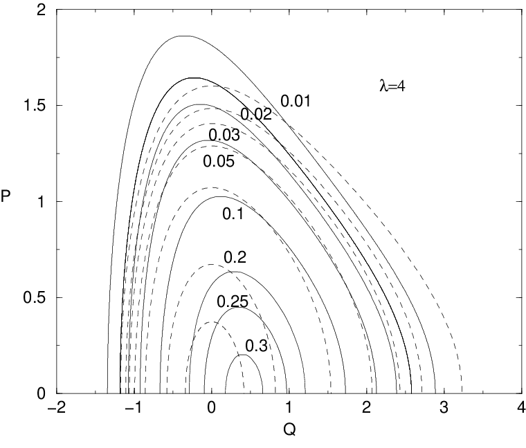
In Figs. 10,11,12 and 13 we present SDF curves for fixed $\rho_{c}$ superposed on WDF curves with $\rho=\rho_{c}$ for comparison. It will be seen that, as $\lambda$ increases the SDF approximation improves, which means also that the WDF curves of constant $\rho$ become closer to classical trajectories. In Fig. 9 we plot curves of constant $\rho_{c}$ for the case $\lambda=1$. For this oscillator our semiclassical approximation is anomalous, as the value of $\rho_{c}$ increases from $\rho_{c}=0.145$ to $\rho_{c}=0.179$ as the classical energy $E$ varies from $E=0$ to $E=0.26\hbar\omega_{0}$ but decreases as $E$ increases further. For the other oscillators $\rho_{c}$ decreases as the energy $E$ increases until reaching the value $\rho_{c}=0$. As a consequence for $\lambda=1$ one has two closed curves with the same $\rho_{c}$ for $0.145<\rho_{c}<0.179$ whereas for $\lambda\geq 2$, for each $\rho_{c}$ one has only one such curve. Also for the WDF there is only one closed curve for each $\rho$ from the maximum value of $\rho$ up to the curve $\rho=0$.

In Fig. 10 we compare the WDF curves of constant $\rho$ with the SDF curves for which $\rho=\rho_{c}$ in the case $\lambda=1$. One notices that the discrepancies between both curves are very large. In Figs. 11,12 and 13 we make the same comparison for $\lambda=2,4$ and 10 respectively.

One finds that for $\rho<0.05$ both curves are quite similar but displaced from each other. This displacement becomes less pronounced as $\rho$ gets closer to 0.05 so that the best agreement between $\rho$ and $\rho_{c}$ is reached for $\rho\approx 0.05$. Also as $\lambda$ increases the displacement between both curves decreases, as it can be seen comparing the oscillators $\lambda=4$ and $\lambda=10$. For $\rho\stackrel{{\scriptstyle>}}{{\sim}}0.05$ the curves of fixed $\rho_{c}$ compared with the curves of fixed $\rho$ contain a certain amount of distortion which becomes less pronounced as $\lambda$ increases.

Finally we observe that curves with $\rho_{c}=0.3$ are absent, the largest values of $\rho_{c}$ being 0.227, 0.271 and 0.299 respectively for $\lambda=2,4$ and 10, values which are reached at the origin of phase-space.

References

• [1] E. Wigner, Phys. Rev. 40, 749 (1932).
• [2] H. W. Lee and M. O. Scully, J. Chem. Phys. 77(9), 4604 (1982).
• [3] G. W. Bund, J. Phys. A28 3709 (1995).
• [4] G. W. Bund and M. C. Tijero, Phys. Rev. A 61, 052114 (2000).
• [5] P. M. Morse, Phys. Rev. 34, 57 (1929).
• [6] J. P. Dahl and M. Springborg, J. Chem. Phys. 88(7), 4535 (1988).
• [7] A. Frank et al, Ann. Phys. (N.Y.) 252, 211 (1996).
• [8] J. P. Dahl, in Semi-classical Descriptions of Atomic and Nucleon Collisions, J. Bang and J. de Boer (Eds.) (Elsevier Science Publishers, B.V. 1985).
• [9] W. C. De Marcus, Am. J. Phys. 46, 733 (1978).
• [10] S. R. Groot and L. G. Suttorp, in Foundations of Electrodynamics (Amsterdam: North-Holland, 1972).
• [11] M. M. Nieto and L. M. Simmons Jr. Phys. Rev. A 19, 438 (1979).
• [12] D. ter Haar, Problems in Quantum Mechanics, 3th Edition (Pion, London, 1975).
Refer to caption
Figure 1: The Morse potential V⁡(Q)V(Q) defined by Eq. (39c) and the corresponding bound-state energies EnE_{n} given by Eq. (39d), for λ=1\lambda=1.
Figure 2: Same as Fig. 1 for λ=2\lambda=2.
Figure 3: Same as Fig. 1 for λ=4\lambda=4.
Figure 4: Same as Fig. 1 for λ=10\lambda=10.
Figure 5: Curves of constant Wigner distribution function ρ⁡(Q,P)\rho(Q,P) in units of ℏ−1\hbar^{-1} for the ground state of the Morse oscillator with λ=1\lambda=1.
Figure 6: Same as Fig. 5 for λ=2\lambda=2.
Figure 7: Same as Fig. 5 for λ=4\lambda=4.
Figure 8: Same as Fig. 5 for λ=10\lambda=10.
Figure 9: Curves of constant semi-classical distribution function ρc​(Q,P)\rho_{c}(Q,P) in units of ℏ−1\hbar^{-1} for the ground state of the Morse oscillator with λ=1\lambda=1. For 0.145<ρc<0.1790.145<\rho_{c}<0.179 one has two curves for each value of ρc\rho_{c}.
Figure 10: Full curves are curves with a constant value of the Wigner distribution function ρ\rho and dashed lines have constant value of the semiclassical distribution function ρc\rho_{c} for the ground state of the Morse oscillator with λ=1\lambda=1. Except for ρ=0.2\rho=0.2, for each full line with a given ρ\rho one has one or two corresponding dashed lines with ρc\rho_{c} such that ρc=ρ\rho_{c}=\rho.
Figure 11: Same as Fig. 10 for λ=2\lambda=2. Except for ρ=0.3\rho=0.3 and ρ=0.25\rho=0.25, for each full line one has a corresponding dashed line with ρc\rho_{c} such that ρc=ρ\rho_{c}=\rho.
Figure 12: Same as Fig. 10 for λ=4\lambda=4. Except for ρ=0.3\rho=0.3, for each full line one has a corresponding dashed line with ρc\rho_{c} such that ρc=ρ\rho_{c}=\rho.
Figure 13: Same as Fig. 10 for λ=10\lambda=10. Except for ρ=0.3\rho=0.3, for each full line one has a corresponding dashed line with ρc\rho_{c} such that ρc=ρ\rho_{c}=\rho.