On deciding whether a Boolean function is constant or not Work supported in part by Istituto Nazionale di Fisica Nucleare, Sezione di Trieste, Italye-mail: marinatto@ts.infn.it

This task is successfully achieved by exploiting two essential features of quantum mechanics: its linearity, which allows the simultaneous evaluation of a function on linear superpositions of its input values, and the interference between amplitudes, which raises the probability of obtaining the desired results.

The a-priori knowledge that the function computed by the quantum oracle is either constant or balanced, is crucial in solving the problem exactly, i.e. with zero probability of error. In this paper, we address the question of deciding the constancy of a generic function chosen at random among the set of $2^{2^{n}}$ $n$-bit Boolean functions. In such a case, the iteration of the same algorithmic procedure permits one to decide about the constancy of such generic function with a probability of error which depends on $n$ and on the number $k$ of quantum oracle-queries.

Unfortunately, this probability tends to $1$ in the worst case scenario, namely when the given function outputs the same value for every input but one. Nevertheless, it is our purpose to determine the efficiency of the quantum algorithm and the range of values of $n$ and $k$ for which it is more efficient compared to the unique classical procedure which involves querying the oracle successively until two different outputs are encountered.

Not too surprisingly, due to classical conditioning of each output on the previous ones, in some specific situations (the worst cases), for large number of inputs and nearly as many oracle-queries, the efficiency of the classical algorithm turns out to overcome that of the quantum one. Moreover, in the average case, i.e. when the $n$-bit Boolean function is sorted at random, the quantum algorithm is always preferable to the classical one.

The general problem we are going to tackle is as follows. Suppose that we are given an oracle which instantaneously computes an arbitrary n-bit Boolean function $f\,:\,\left\{0,1\right\}^{n}\rightarrow\left\{0,1\right\}$ on inputs that, as usual, will be enumerated by the integers $\left\{0,1,\dots,2^{n}-1\right\}$. Our goal is to devise a quantum algorithm, involving oracle queries, in order to determine, with some probability of error, whether such a function is constant or not.

Since, by hypothesis, we have no a-priori information or knowledge about $f$, we can only suppose that it has been sorted completely at random within the set ${\cal{S}}_{n}$ of $2^{2^{n}}$ n-bit Boolean functions.

If we have at our disposal a classical oracle which outputs the value of $f$, and which can be queried at most $k$ times, the only conceivable classical algorithm able to solve the problem is : ‘‘query the oracle $k$ times or until two output values are different: in the latter case stop querying and declare that the function is not constant, otherwise say that $f$ is constant”.

Of course, this simple algorithm fails to give the right answer only when the function is actually non-constant and when we have obtained $k$ consecutive equal digits in the querying procedure. In fact, the function $f$ might output a different digit on any of the untried inputs, so that one has to evaluate the probability of such an event.

We start by considering the worst possible scenario, that is the unknown function $f$, drawn from the set ${\cal{S}}_{n}$, actually outputs the same bit, say $0$, for all of its inputs but one (for simplicity of notation we will say that such a function is of $f_{1}$-type). The probability $p_{1}(k,n)$ of declaring erroneously constant such a function, coincides with the probability of obtaining $k$ consecutive digits $0$ after querying the oracle $k$ times:

$$p_{1}(k,n)=\textrm{Prob}[\underbrace{0\dots 0}_{k}]=\textrm{Prob}[0]\cdot\Big(\prod_{\ell=1}^{k-1}\textrm{Prob}[\,0|\underbrace{0\dots 0\,}_{\ell}]\Big),$$

(2.1)

where we have indicated with $\textrm{Prob}[\,0|\underbrace{0\dots 0\,}_{\ell}]$, $1\leq\ell\leq k-1$, the conditional probability of getting $0$ after the $(\ell+1)$-th oracle query if a sequence of $\ell$ consecutive zeroes has already been obtained. Since the function $f$ is of $f_{1}$-type, one easily calculates $\textrm{Prob}[0]=(2^{n}-1)/2^{n}$ and $\textrm{Prob}[0|\underbrace{0\dots 0\,}_{\ell}]=(2^{n}-\ell-1)/(2^{n}-\ell)$, whence

$$p_{1}(k,n)=\prod_{j=1}^{k}\frac{2^{n}-j}{2^{n}-(j-1)}=1-\frac{k}{2^{n}}\>.$$

(2.2)

This probability distribution is equal to zero for $k=2^{n}$; indeed, due to statistical correlations between subsequent outputs, in such a case we can determine with certainty if the function is constant or not. As we will see, this is not the case with the Deutsch-Josza quantum algorithm which, unless the function is either constant or balanced, is not able to give the correct answer with certainty. First, let us briefly recall the basics of that algorithm whose associated quantum circuit is the following:

We denote by $q_{1}(k,n)$ the probability that, after obtaining $z=0$ in $k$ consecutive measurements, we are wrong in asserting the constancy of the $f_{1}$-type function. According to Eq. (2.5), one gets:

$$q_{1}(k,n)=\Big(1-\frac{1}{2^{n-1}}\Big)^{2k}\>.$$

(2.6)

It is worth noting that, contrary to the classical case where the probability of obtaining the same output value changes, by conditioning, after each oracle query, the consecutive (quantum) oracle-queries are independent from each other. Therefore, the probability of obtaining $z=0$, $k$ times consecutively, is the product of the probabilities of the uncorrelated events; quantum conditioning on past results would certainly improve the efficiency of the algorithm, however we do not know of any such technique.

In order to compare the quantum querying procedure with respect to the classical one in this worst case, we define the following efficiency function $\Delta_{1}(k,n)$:

$$\Delta_{1}(k,n)\equiv p_{1}(k,n)-q_{1}(k,n)=1-\frac{k}{2^{n}}-\Big(1-\frac{1}{2^{n-1}}\Big)^{2k}\>.$$

(2.7)

Given $n$ (the number of bits) and $k$ (the number of oracle-queries), a positive value of $\Delta_{1}(k,n)$ indicates that the quantum algorithm is more efficient than the classical one. For $n\geq 2$ and $1\leq k\leq 2^{n}-1$, $\Delta_{1}(k,n)$ attains its absolute maximum at $n=2$ and $k=1$:

$$\max_{k,n}\>{\Delta_{1}(k,n)}=\Delta_{1}(k=1,n=2)=0.5\>\>.$$

(2.8)

For fixed $n$, the function $\Delta_{1}(k,n)$ has relative maxima at

$$k^{\star}\cong 0.5\,\frac{\log{\Big(-\frac{2^{-1-n}}{\log{(1-2^{1-n})}}}\Big)}{\log{(1-2^{1-n})}}\>\approx\>\>0.35\cdot 2^{n}\>\>\>\>\>\>\textrm{for}\>\>2^{n}\gg 1\>,$$

(2.9)

with $\Delta_{1}(k^{\star},n)\approx 0.40$, for $2^{n}\gg 1$.

In Fig. 1, $\Delta_{1}(k,n)$ is plotted as a function of $k$ for different values of $n$; the curves displayed from left to right are associated with increasing values of $n$, $5\leq n\leq 12$:

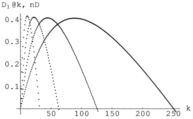
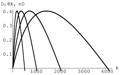
As it can be argued from the picture plotted above, $\Delta_{1}(k,n)$ is a concave function in the variable $k$ for every fixed value of $n\geq 3$. Therefore, the worst case efficiency of the quantum algorithm increases, with respect to the classical one, for $k\leq k^{\star}$ (where $k^{\star}\approx 0.35\cdot 2^{n}$ for $2^{n}\gg 1$), until it reaches its (relative) maximum value. Such a value exhibits a weak dependence on the variable $n$ and it is approximately equal to $0.40$ for $2^{n}\gg 1$. On the contrary, for $k>k^{\star}$, $\Delta_{1}(k,n)$ decreases to zero, thus indicating a substantial equivalence of the two methods for large $k$’s.

The above results show that, in the worst case, it is almost always better to resort to the quantum rather than to the classical algorithm. However, the improvement of quantum queries over the classical ones decreases with the number of queries. Furthermore, $\Delta_{1}(k,n)$ becomes negative for $k\cong 2^{n}$, namely there is a (small) range of values of $k$ for which the classical querying procedure gives less probability of error than the quantum one.

Not surprisingly, this is due to the fact that the $2^{n}$-th classical query is able to determine with certainty if the function is constant or not, since $p_{1}(k=2^{n},n)=0$. Instead, the quantum algorithm, as it has been conceived, can never answer with certainty since $q_{1}(k,n)$ never vanishes.

Until now we have restricted our analysis to the worst possible scenario, i.e. when the function $f$ outputs the same value for all possible inputs but one. In the general case, the function may be any of the $2^{2^{n}}$ possible $n$-bit Boolean functions belonging to the set ${\cal{S}}_{n}$. This set contains $2$ constant functions (one always outputs $0$, while the other outputs $1$), ${2^{n}\choose 2^{n-1}}$ balanced functions (they output the same value for exactly one-half of the possible inputs) and $2\cdot{2^{n}\choose 2^{n}-m}$ $f_{m}$-type functions (they output $0$ ($1$) on $2^{n}-m$ inputs and $1$ ($0$) on the remaining $m$ ones).

We repeat the analysis of the previous section and suppose we are given one particular $f_{m}$-type function. The probability of obtaining always the same output bit by querying the classical oracle $k$ times, and thus of concluding, erroneously, that the function is constant, is equal to $\textrm{Prob}[\underbrace{0\dots 0}_{k}]+\textrm{Prob}[\underbrace{1\dots 1}_{k}]$. The latter are the probabilities of obtaining $k$ consecutive digits $0$ and $1$ respectively, and they explicitly read

$$\textrm{Prob}[\underbrace{0\dots 0}_{k}]=\prod_{j=0}^{k-1}\frac{2^{n}-m-j}{2^{n}-j}=\frac{(m-2^{n})_{k}}{(-2^{n})_{k}}\>,$$

(3.1)

$$\textrm{Prob}[\underbrace{1\dots 1}_{k}]=\prod_{j=0}^{k-1}\frac{m-j}{2^{n}-j}=\frac{(-m)_{k}}{(-2^{n})_{k}}\>.$$

(3.2)

In the above, for simplicity of notation, the Pochhammer symbol $(a)_{n}\equiv a(a+1)\dots(a+n-1)$ has been used. Therefore, the classical error probability $p_{m}(k,n)$ in declaring constant an $f_{m}$-type function is:

$$p_{m}(k,n)=\frac{(m-2^{n})_{k}}{(-2^{n})_{k}}+\frac{(-m)_{k}}{(-2^{n})_{k}}.$$

(3.3)

The corresponding probability $q_{m}(k,n)$ for the quantum case is much easier to calculate. In fact, given an $f_{m}$-type function, the conditional probability of obtaining $k$ consecutive measurement results $z=0$ via the iterated Deutsch-Jozsa procedure is, according to Eq. (2.4):

$$\textrm{Prob}[k\>\textrm{times}\>z\!=\!0,{\bf|}\,f\!=\!f_{m}]\equiv q_{m}(k,n)=\Big|\frac{1}{2^{n}}\sum_{x=0}^{2^{n}-1}(-1)^{f(x)}\Big|^{2k}=\Big(1-\frac{m}{2^{n-1}}\Big)^{2k}\>.$$

(3.4)

As in the previous section, we can now define a function $\Delta_{m}(k,n)$ which quantifies the relative efficiency of the quantum algorithm with respect to the classical one:

$$\Delta_{m}(k,n)\equiv p_{m}(k,n)-q_{m}(k,n)=\frac{(m-2^{n})_{k}}{(-2^{n})_{k}}+\frac{(-m)_{k}}{(-2^{n})_{k}}-\Big(1-\frac{m}{2^{n-1}}\Big)^{2k}\>.$$

(3.5)

$\Delta_{m}(k,n)$ does not dramatically change with $n$; therefore, we fix $n\!=\!7$ and present typical behaviours for different values of $m$.

We notice that $\Delta_{m}(k,n)$ is symmetric around $m=2^{n-1}$, and that, when $m$ gets close to $2^{n-1}$, the function $f_{m}$ tends to be balanced and $\Delta_{m}(k,n)$ rapidly decreases. This behaviour indicates that the quantum algorithm can perform much better than the classical one, but only for small numbers of oracle-queries. On the contrary, the two procedures become equally efficient for larger values of $k$. For instance, in Fig. 2, when $m=60$ and the function $f_{m}$ is almost balanced, the two procedures are nearly indistinguishable for $k>5$. Instead, in the general case of $m$ significantly different from $2^{n-1}$, the dependence of $\Delta_{m}(k,n)$ on $k$ is much smoother and presents a maximum and a change of concavity. Further, for $k\cong 2^{n}$, $\Delta_{m}(k,n)$ assumes negative values, invisible in the above pictures. This indicates a better performance of the classical algorithm over the quantum one, as already noticed when dealing with the $f_{1}$-type function in the previous section. However this phenomenon is much less pronounced than in the worst case situation.

In this paper we have shown how a trivial iteration of the original Deutsch-Jozsa algorithm, can be applied to solve the general problem of deciding if a function $f$, sorted at random among the set of $n$-bit Boolean functions, is constant or not. We have compared the error probability of the quantum procedure with that of the classical one, the latter consisting of consecutive oracle-queries performed until two different outputs are encountered. We have analyzed the range of values of $n$ and $k$ for which the quantum procedure is more efficient than the classical one, both on average and in the worst possible situation. From a numerical analysis, one concludes that, by iterating the quantum algorithm, one can always solve the problem, on average, better than with the classical method, and much better in those situations where the number of queries $k$ is small and $2^{n}$ large. Moreover, we have seen that, when $f$ is a $f_{m}$-type function with $m$ not much greater than $1$ (the worst cases), then the classical method is asymptotically (that is, when $2^{n}$ is large and $k\cong 2^{n}$) preferable to the quantum one. This peculiar effect is due to the fact that the Deutsch-Jozsa algorithm, unlike the classical querying, can never solve the general problem with certainty since it does not allow for conditioning on previous results.

References

- [1] R.Beals, H.Buhrman, R.Cleve, M.Mosca and R. de Wolf; “Quantum lower bounds by polynomials”, in Proceedings of the 39th Annual Symposium on Foundations of Computer Science (FOCS’98), IEEE, (1998).
- [2] E.Farhi, J.Goldstone, S.Gutmann, M.Sipser; “Limit on the speed of quantum computation in determining parity”, Phys. Rev. Lett., 81, 5542-5444, (1998).
- [3] W. van Dam; “Quantum oracle interrogations: getting all information for almost half the price”, in Proceedings of the 39th Annual Symposium on Foundations of Computer Science (FOCS’98), IEEE, (1998).
- [4] D.Deutsch and R.Jozsa; “Rapid solution of problems by quantum computation”, Proc. R. Soc. London A, 439, 553-558 (1992).