Full quantum solutions to the resonant four-wave mixing of two single-photon wave packets
Abstract
We analyze both analytically and numerically the resonant four-wave mixing of two co-propagating single-photon wave packets. We present analytic expressions for the two-photon wave function and show that soliton-type quantum solutions exist which display a shape-preserving oscillatory exchange of excitations between the modes. Potential applications including quantum information processing are discussed.
pacs
42.50, 42.65, 03.67-aI Introduction
The cancellation of resonant linear absorption and refraction via electromagnetically induced transparency (EIT) harris1997; Marangos has led to a range of new possibilities in non-linear optics. One important application is optical frequency mixing close to atomic resonances which allows the use of the enhanced nonlinear interaction without suffering from linear absorption and refraction. It has been predicted that EIT could lead to a new regime of nonlinear optics on the level of few light quanta Harris1998; HauHarris99; Imamoglu96; Lukin-AdvAMO-2000; johnsson2002a. Several schemes for resonant nonlinear processes have been proposed and analyzed, both theoretically and experimentally Lukin-AdvAMO-2000. A particularly interesting system is resonant four-wave mixing using atoms with a double-lambda configuration Hemmer1994; Babin1996; Popov1997; Lu1998. Efficient frequency conversion, generation of squeezing LukinPRL1999 as well as the possibility of mirrorless oscillations Lukin1998 with extremely low thresholds and narrow linewidth have been predicted Fleischhauer-PRL-1999 and in part experimentally observed Zibrov-PRL-2000.
Most theoretical and experimental studies of resonant nonlinear processes have been done for classical fields. For one-dimensional set-ups where common co-moving frames exist, full analytical solutions have been derived for the interaction of classical pulses in the adiabatic limit Korsunsky2002. In view of the potential for an efficient nonlinear interaction on the level of few photons, however, a full quantum theoretical analysis of these systems is necessary. In addition, in order to take into account finite size effects which become increasingly important in the few-photon regime, and to analyze the potential for quantum information processing, such a quantum analysis has to go beyond the usual linearization approaches. Here very little work has been done, the few exceptions being the integrable models of resonantly enhanced Kerr interaction Imamoglu-Kerr and photon blockade Harris1998; blockade.
In a previous paper johnsson2002a we have shown numerically that if single-mode fields are considered, it is possible to use an atomic vapor in a four-wave mixing double-lambda configuration to obtain full conversion from two input fields into two generated fields within a few centimeters of interaction length, even if the input fields only consist of single light quanta. The treatment was fully quantum but being restricted to a single-mode analysis, propagation effects of wave packets were not considered. In the present paper we extend this study by undertaking a multimode analysis in one spatial dimension and for co-propagating fields. In order to keep the problem tractable we restrict ourselves to the important special case of two single-photon wave packets as inputs. For this case we obtain simple analytic solutions and compare them to numerical simulations. We show that soliton-like quantum solutions exist that display an oscillatory exchange of excitation between the two input and the two generated fields. Finally we discuss briefly possible applications of single-photon four-wave mixing to quantum information processing and entanglement generation.
II System and effective field equations
The situation we consider is resonantly enhanced four-wave mixing in the modified double-lambda system shown in Fig. 1. Note that a five-level atomic system is used instead of the original four-level system put forward in Hemmer1994; Lukin1998. This is due to the fact that in the four-level system the finite detuning is associated with an AC Stark effect, which leads to intensity dependent dynamical phase shifts of the fields. These phase shifts are of minor consequence in the case where the fields are counter-propagating Fleischhauer00b, but for co-propagating fields have a detrimental influence leading to impaired phase matching and inefficient frequency conversion. As shown in johnsson2002b these phase shifts are eliminated in the five-level scheme when the relative sign of the dipole moments of the transitions is opposite to that of the transitions.
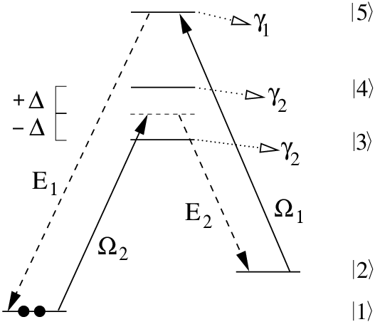
The two fields with carrier frequencies and and slowly varying amplitudes and are initially excited and form the pump fields. The other fields of carrier frequencies and and slowly varying amplitudes and are generated during the interaction process and are assumed to be initially zero. and are taken to be exactly on resonance, i.e. , , while the other two fields are detuned by an amount , i.e. and . A finite detuning , large compared to the Rabi frequencies, the Doppler broadening and the decay rates from the excited states, is necessary to maximize the ratio of nonlinear gain to linear absorption. Decay from the two lower levels is considered to be negligible and all fields have the same propagation direction.
Because of energy conservation there is overall four-photon resonance, i.e. . It can be shown that the contributions of the resonant transitions to the linear refractive index vanish if the fields are pairwise in two-photon resonance. Phase matching will thus favor two-photon resonance and we assume that this condition is fulfilled for the carrier frequencies of the four pulses, i.e. .
Extending the analysis of johnsson2002a to a multimode description, the interaction can be described by the effective adiabatic Hamiltonian hamiltonian
| (1) |
Here etc. denote dimensionless, slowly-varying (both in time and space) positive and negative-frequency components of the corresponding electric fields
| (2) | |||||
| (3) |
is the quantization length and is the wave-vector component in -direction relative to . The four fields are assumed to have either sufficiently different carrier frequencies or different polarizations. Thus operators corresponding to different fields commute. The commutator between positive and negative frequency components can be approximated by a spatial delta function
| (4) |
We furthermore assume in (1) that all four transitions give rise to the same coupling , where is the atomic number density, the typical wavelength of the fields and the typical radiative decay rate. It should be noted that numerator and denominator of Eq. (1) commute and thus there is no ambiguity with respect to the ordering of the terms.
The structure of the denominator results from the saturation of the two-photon transition , whose coherence lifetime is taken to be infinite. If a finite decay rate of the coherence is taken into account, a term proportional to has to be added in the denominator.
The non-polynomial character of the interaction Hamiltonian causes the nonlinear coupling to behave unusually: As shown in johnsson2002a, the interaction increases with decreasing pump field strength, making effective nonlinear frequency conversion possible even for single photons. In the derivation of the effective Hamiltonian in johnsson2002a adiabatic conditions were assumed. This limits the applicability of (1) in the multimode case to sufficiently long pulses. A discussion of non-adiabatic corrections and their effect on the propagation of the pulses is, however, outside of the scope of the present paper and will be discussed elsewhere.
As shown in the Appendix the slowly varying amplitudes of the electric field obey
| (5) |
and similarly for . Thus from (1) we arrive at the following equations of motion
| (6) |
where and .
These equations admit four independent constants of motion:
| (7) |
which represent the quantum analogs of the Manley-Rowe relations and additionally the conservation of the relative phase between the fields.
If we assume that the input fields consist of two, single-photon wave packets in and , then it is clear, due to the constants of motion (7), that the state of the system can be represented at all times by
| (8) |
where denotes photons in the th mode of , photons in the th mode of , and so on.
III Field intensities
Since for the case of a single-photon input the expectation values of all fields vanish at all times, all relevant information about the state of the system is given by the mean intensities of the fields
| (9) |
and the two-photon wave functions
| (10) | |||||
| (11) | |||||
and represent the amplitude of finding the () photon at position and simultaneously the () photon at position . The ’s are 2D Fourier transforms from the -space representations and into a real-space representation.
We first discuss the dynamics of the mean intensities of the fields. Due to the constants of motion it is sufficient to calculate say .
| (12) | |||||
where we have dropped the common spatial coordinate and used , as well as the fact that three annihilation operators acting on give zero. Similarly we find
| (13) | |||||
| (14) | |||||
Consequently the differential equation we must solve is
| (15) |
We take the input to be two independent single-photon wave packets in and with the same spatial envelope and vacuum in the other two fields, which corresponds to a separable initial state of the form
| (16) | |||||
The are Fourier-transforms of
| (17) |
Thus
| (18) | |||||
where . With these initial conditions one finds
| (19) |
i.e. a sinusoidal exchange of excitation between the two pump and the two generated fields. Complete conversion is achieved at . It is worthwhile noting that as shown in johnsson2002a, and contrary to the classical dynamics, complete conversion can only be achieved in the quantum case for initial Fock states with one or two photons in the two pump modes.
IV Dynamics of the two-photon wave function; quantum solitons
We proceed by calculating the two-photon wave functions. The calculation of can be split into two distinct cases, depending on whether or . Let us first assume .
| (20) | |||||
where we have again used the results that , and that three annihilation operators acting on give zero. Operating on we find
| (21) |
Thus, to determine the wave function, we need to solve the differential equation
| (22) |
For an input consisting of two independent single-photon wave packets with the same spatial shape, as considered above, the initial two-photon wave function reads
| (23) |
We also have at the entrance of the medium
| (24) |
so that the solution to (22) is given by
| (25) |
with . Thus the two-photon wave function at equal spatial points propagates through the medium modulated by a factor of . We see that after one full conversion cycle the phase of the wave function has changed sign. This agrees with a numerical simulation of the quantum problem, the results of which are shown in Fig. 2.

We can use a similar procedure to find , the wave function of the generated fields. We obtain
| (26) |
The evolution of this field is shown in Fig. 3. Note that it is out of phase with the drive field wave functions, as expected.

For full knowledge of the state of the system, we also need to find where . From (4) we see that operators at different points in space commute, so that
| (27) | |||||
Expanding the Hamiltonian, normal ordering the expression and again noting the form of (8) we eventually arrive at
| (28) |
Thus the wave function of the system in the case where is simply given by the corresponding input expression
| (29) |
It is evident that the initial two-photon wave function at different coordinates propagates undisturbed throughout the medium, and that there is a discontinuous change in the behavior when moving away from the line . This is clearly seen in Fig. 4, which shows the two dimensional wave function at time . This is the time required for one full conversion from the pump fields to the generated fields and back again. Essentially we have at this time
| (30) | |||||
| (31) |

This behavior can easily be understood. The two-photon wave function represents the joint probability density that two photons are located at positions and . As both photons propagate at the same speed they will never meet at the same point in space unless they did initially. Since the nonlinear interaction in (1) is local, two photons at different spatial points do not interact. Thus only if is there a conversion from the pump fields into the generated fields due to the local nonlinearity.
The simple sign change in the wave function for hints at the possibility of using the system as a phase gate for quantum computation, as was mentioned in the single-mode case considered in johnsson2002a. One chooses the length of the nonlinear medium such that exactly one full conversion cycle can occur. If the entire wave function changes sign, we would have a system that behaves as a true phase gate: if only one of the two inputs is populated, the pulse exits the medium unchanged, but if both are present, a phase shift of occurs.
However, due to the multimode nature of this problem, it is for all and that is a true reflection of the system rather than and there is no sign change for . To see whether we can still use the system as an approximate phase gate, we consider the behavior of the state vector coefficients in (8). Returning briefly to a picture with discrete modes, by using Eq. (38) of the Appendix one can show that (30) and (31) imply
| (32) |
This gives a good picture of how the different modes have mixed among themselves, and shows that in general a simple sign change of all the coefficients cannot exist. Only if we can enforce that at least temporarily only a single effective mode of the two pump fields is excited, e.g. by using a resonator set-up is it possible to use the system as a phase gate.
We see however from (32) that after one full conversion cycle the initially factorized state (16) evolves into an entangled state between all modes of the fields and . Thus the nonlinear interaction generates entanglement.
On the other hand if the initial state is a two-photon wave packet in an entangled state, such that the initial two-photon wavefunction has only a contribution for
| (33) |
only diagonal components of the two-photon wave function will ever be nonzero. According to (25) and (26) they undergo sinusoidal oscillations
| (34) | |||||
| (35) |
The superposition of pump and generated fields
| (36) | |||||
propagates in a form-stable manner and represents a quantum soliton solution. The two-photon wavefunction of the quantum soliton corresponds to a quasi-particle excitation
| (37) | |||
V summary
In the present paper we have presented a full quantum theoretical treatment of resonant forward four-wave mixing for pulses. For this we have used an effective Hamiltonian derived from the interaction of the fields with an ensemble of atoms in a double-lambda configuration using an adiabatic approximation johnsson2002a. We were particularly interested in the few-photon regime since here quantum effects dominate the dynamics and because of potential applications in quantum information processing. Thus we have restricted ourselves to the important special case of an input consisting of two single-photon wave packets. For this case we were able to analytically solve the propagation equations for the field intensities and two-photon wave functions which contain all relevant information about the quantum state.
We found that there is an oscillatory energy exchange between the two pump and generated fields with 100% conversion at periodic intervals of interaction. This result is characteristic for a few-photon Fock-state input; for a coherent input complete conversion can only be achieved asymptotically for very large input power.
We have also shown that after even multiples of the conversion length the two-photon wave function regains its initial form, while after odd multiples there is a sign flip for .
If the two input wave packets are not independent but in a highly entangled state, the two-photon wave function can be made zero outside of the diagonal. It was shown that such a pair of input wave packets form a formstable soliton-like quantum solution which is a superposition of pump and generated fields with oscillating coefficients.
The process of resonant four-wave mixing was shown to generate large entanglement between the modes forming the two, single-photon wave packets. Furthermore the nonlinear interaction strength is large enough to generate a controlled phase shift of a single photon by the presence of another one. Thus, if the number of relevant modes is at least temporarily restricted by some external means like a resonator, the system could have interesting applications as a photonic phase gate.
Acknowledgement
The authors acknowledge financial support by the Deutsche Forschungsgemeinschaft through the special program on quantum information and the Graduiertenkolleg 792 at the University of Kaiserslautern.
Appendix
To simplify the transition from a single-mode description to a multimode one, we will first consider one single-mode quantum field , and then generalize the result to our four-field system. Suppose that the single-mode Hamiltonian governing the evolution of is given by . To go over to the multimode description we consider an interaction region of length , divided into cells, and consider a discrete set of modes around the carrier frequency of the field, i.e. , . We now define localized field operators (denoted by a tilde) via
| (38) | |||||
| (39) |
where the are annihilation operators for mode . is related to the field strength in cell .
These localized field operators have the commutation relations
| (40) |
The multimode Hamiltonian can now be written as
| (41) | |||||
where is the carrier frequency and
| (42) |
Commutation relations yield the following Heisenberg equation of motion
| (43) |
Now, as we let we find
| (44) | |||||
| (45) | |||||
| (46) | |||||
| (47) |
Introducing slowly time-varying amplitudes we obtain
| (48) |
Thus the multimode equations of motion look exactly like the single-mode equations of motion with the exception that a term has been added and the fields now have a spatial dependence.
Returning to the four-wave mixing situation described in this paper, we see that the interaction Hamiltonian given by (1) is of the form shown above, with the summation replaced by an integral in the continuum limit. The multimode annihilation and creation operators and defined in (2) and (3) are analogous to the localized field operators defined above, except for the factor of inserted to ensure correct commutation relations regardless of the quantization length. Thus the equation of motion (5) follows from (48) above.
References
- (1) S. E. Harris, Physics Today 50, 36 (1997).
- (2) E. Arimondo, Prog. in Optics, 35, 259 (1996), P. L. Knight, B. Stoicheff and D. F. Walls (eds.), Phil. Trans. R. Soc. Lond. A 355, 2215-2416 (1997), J. P. Marangos, Journal of Modern Optics, 45, 471 (1998),
- (3) S. E. Harris and Y. Yamamoto, Phys. Rev. Lett. 81, 3611 (1998)
- (4) M. Jain, Hui Xia, G. Y. Yin, A. J. Merriam, and S. E. Harris, Phys. Rev. Lett. 77, 4326 (1996); S. E. Harris and L. V. Hau, Phys. Rev. Lett. 82, 4611 (1999)
- (5) H. Schmidt and A. Imamoglu, Opt. Lett. 21, 1936 (1996), M. D. Lukin and A. Imamoglu, Phys. Rev. Lett. 84, 1419 (2000).
- (6) M.D. Lukin, P.R. Hemmer, and M.O. Scully, Adv. Atom. Mol. Opt. Phys. 42, 347 (2000).
- (7) M.T. Johnsson, and M. Fleischhauer, Phys. Rev. A 66, 043808 (2002).
- (8) P.R. Hemmer, K. Z. Cheng, J. Kierstead, M. S. Shariar, and M. K. Kim, Opt. Lett. 19, 296 (1994); B. S. Ham, M. S. Shariar, M. K. Kim, and P. R. Hemmer, Opt. Lett. 22, 1849 (1997).
- (9) S. Babin, U. Hinze, E. Tiemann, B. Wellegehausen, Opt. Lett. 21, 1186 (1996); S. Babin, E. V. Podivilov, D.A. Shapiro, U. Hinze, E. Tiemann, B. Wellegehausen, Phys. Rev. A 59, 1355 (1999); U. Hinze, L. Meyer, B.N. Chichkov, E. Tiemann, B. Wellegehausen, Opt. Comm. 166, 127 (1999).
- (10) A. K. Popov, S. A. Myslivets, Kvant. Elektr. 24, 1033 (1997).
- (11) B. Lu, W.H. Burkett, M. Xiao, Opt. Lett. 23, 804 (1998);
- (12) , M.D. Lukin, A.B. Matsko, M. Fleischhauer, and M.O. Scully, Phys. Rev. Lett. 82, 1847 (1999).
- (13) M. D. Lukin, P. R. Hemmer, M. Löffler and M. O. Scully Phys. Rev. Lett. 81, 2675 (1998); A. S. Zibrov, M. D. Lukin and M. O. Scully Phys. Rev. Lett. 83, 4049 (1999).
- (14) M. Fleischhauer, M. D. Lukin, A. B. Matsko, and M. O. Scully, Phys. Rev. Lett. 84, 3558 (2000).
- (15) A.S. Zibrov, M.D. Lukin, and M.O. Scully, Phys. Rev. Lett. 83, 4049 (1999).
- (16) E. A. Korsunsky and M. F. Fleischhauer, Phys. Rev. A 66, 033808 (2002).
- (17) M. D. Lukin and A. Imamoğlu, Phys. Rev. Lett. 84, 1419 (2000).
- (18) A. Imamoğlu, H. Schmidt, G. Woods, and M. Deutsch, Phys. Rev. Lett. 79, 1467 (1997); M. Dunstan, S. Rebic, S. Tan, S. Parkins, M. Collett, and D. F. Walls, in Proceedings: Quantum Communication, Computing, and Measurement 2, edited by: P. Kumar, G.M. D’Ariano, and O. Hirota (Plenum Press, New York, 1999).
- (19) M. Fleischhauer, in Frontiers of Laser Physics and Quantum Optics, ed. by Z. Xu, S. Xie, S.-Y. Zhu and M.O. Scully, pp. 97 - 106 (Springer, Berlin, 2000).
- (20) M. T. Johnsson, E. Korsunsky, and M. Fleischhauer, Opt. Comm. 212 335 (2002).
- (21) A.O. Melikyan and S.G. Saakyan, Zh. Exp.Teor. Fiz. 76, 1530 (1979) [Sov. Phys. JETP 49, 776 (1979)]; A.R. Karapetyan and B.V. Kryzhanovskii, Zh. Exp. Teor. Fiz. 99, 1103 (1991) [Sov. Phys. JETP 72, 613 (1991)]; B. Kryzhanovsky and B. Glushko, Phys. Rev. A 45, 4979 (1992).