跳到论文正文
W Papers独立论文阅读器 arXiv:quant-ph/0303154 论文正文 计算阅读时间 · 0%
引用这篇论文根据当前论文元数据生成,正式投稿前建议核对。


License: Assumed arXiv.org perpetual non-exclusive license
arXiv:quant-ph/0303154v1 [quant-ph] 25 Mar 2003

An Application of
Renormalization Group Techniques
to
Classical Information Theory

Robert R. Tucci Affiliation: P.O. Box 226 Affiliation: Bedford, MA 01730 Email: tucci@ar-tiste.com
August 11, 2026

Abstract

We apply Renormalization Group (RG) techniques to Classical Information Theory, in the limit of large codeword size nn. In particular, we apply RG techniques to (1) noiseless coding (i.e., a coding used for compression) and (2) noisy coding (i.e., a coding used for channel transmission). Shannon’s “first” and “second” theorems refer to (1) and (2), respectively. Our RG technique uses composition class (CC) ideas, so we call our technique Composition Class Renormalization Group (CCRG). Often, CC’s are called “types” instead of CC’s, and their theory is referred to as the “Method of Types”. For (1) and (2), we find that the probability of error can be expressed as an Error Function whose argument contains variables that obey renormalization group equations. We describe a computer program called WimpyRG-C1.0 that implements the ideas of this paper. C++ source code for WimpyRG-C1.0 is publicly available.

1 Introduction

Renormalization Group (RG) techniques [1] are a panoply of techniques that serve to obtain asymptotic limits. RG techniques usually apply to a system with a very large number of degrees of freedom that is described by a partition function ZZ. Most RG techniques comprise an iterative step (i.e., a step which is performed repeatedly) consisting of a decimation followed by a rescaling. Decimation involves reducing the number of degrees of freedom. Rescaling involves rescaling the variables of ZZ so as to bring ZZ to the same form it had before the previous decimation. (Curiously, in Roman times, the word “decimate” meant to kill 1 out of every 10 prisoners. The modern meaning of the word is more like killing 9 out of every 10).

In this paper, we apply RG techniques to Classical Information Theory[2][3] in the limit of large codeword size nn. In particular, we apply RG techniques to (1) noiseless coding (i.e., a coding used for compression) and (2) noisy coding (i.e., a coding used for channel transmission). Shannon’s “first” and “second” theorems refer to (1) and (2), respectively. For (1), we consider the special case of Csiszár-Körner (CK) universal code. For (2), we consider the special case of random encoding and maximum-likelihood (ML) decoding. For these special cases of (1) and (2), we find that the probability of error can be expressed as an Error Function (see Appendix A) whose argument contains variables that obey RG equations.

Of course, there is no unique way of applying RG techniques to Classical Information Theory. The way shown in this paper is new, to our knowledge. Our RG technique uses composition class (CC) ideas, so we call our technique Composition Class Renormalization Group (CCRG). Often, CC’s are called “types” instead of CC’s, and their theory is referred to as the “Method of Types”.

We end this paper by describing the internal algorithms and typical input and output of a computer program called WimpyRG-C1.0 that implements the ideas of this paper. (The 1.0 is the version number. The C before the 1.0 stands for “Classical”, to distinguish this program from a Q (Quantum) version of WimpyRG that we expect to deliver in the future.) C++ source code for WimpyRG-C1.0 is publicly available, at www.ar-tiste.com/WimpyRG.html .

This paper straddles two fields (RG and Classical Information Theory) which are seldom used together within previous literature. It is therefore most likely that the reader is not closely acquainted with both of these fields. To help readers acquainted with only one of these two fields, the author has strived to make this paper as self-contained as reasonably possible.

Before embarking on long, complicated calculations, let us discuss a simple example that illustrates the manner in which we will apply RG ideas to Information Theory in this paper.

We show in this paper that the probability of error for both noiseless and noisy coding can be expressed as an integral of the following type:

I=∫ξ+∞d​x​e−n​f​(x),I=\int_{\xi}^{+\infty}dx\;e^{-nf(x)}\;, (1)

where n>>1n>>1. Suppose f:R​e​a​l​s→R​e​a​l​sf:Reals\rightarrow Reals is a convex (i.e., shaped like a cup ∪\cup) function with a minimum at x0x_{0}. Let Δ​x=x−x0\Delta x=x-x_{0}, Δ​ξ=ξ−x0\Delta\xi=\xi-x_{0}, and F⁡(Δ​x)=f⁡(x)F(\Delta x)=f(x). Then II can be rewritten as

I=∫Δ​ξ+∞d​Δ​x​e−n​F​(Δ​x).I=\int_{\Delta\xi}^{+\infty}d\Delta x\;e^{-nF(\Delta x)}\;. (2)

II can be approximated as follows

I≈e−n​F​(Δ​ξ).I\approx e^{-nF(\Delta\xi)}\;. (3)

This approximation for II is the leading term of an asymptotic expansion. This method of obtaining asymptotic expansions of integrals is usually called Laplace’s Method [4], named after the inventor of the closely related Laplace Transform. Unfortunately, the II-approximation given by Eq.(3) is poor for those Δ​ξ0\Delta\xi_{0} for which F⁡(Δ​ξ0)=0F(\Delta\xi_{0})=0. Indeed, e−n​F​(Δ​ξ0)e^{-nF(\Delta\xi_{0})} is indeterminate because n​F​(Δ​ξ0)=∞⋅0nF(\Delta\xi_{0})=\infty\cdot 0. Our goal is to devise an II-approximation that overcomes this limitation.

Suppose, for example, that FF is quadratic in Δ​x\Delta x:

F⁡(Δ​x)=a2​(Δ​x)2,F(\Delta x)=\frac{a}{2}(\Delta x)^{2}\;, (4)

for some a>0a>0. Then we can do the integration in Eq.(2) exactly in terms of Error Functions (see Appendix A)

I\displaystyle I =\displaystyle= ∫Δ​ξ+∞d​Δ​x​e−n​a2​(Δ​x)2\displaystyle\int^{+\infty}_{\Delta\xi}d\Delta x\;e^{-n\frac{a}{2}(\Delta x)^{2}} (5a)
=\displaystyle= π2​n​a​erfc​(Δ​ξ​n​a2).\displaystyle\sqrt{\frac{\pi}{2na}}{\rm erfc}\left(\Delta\xi\sqrt{\frac{na}{2}}\right)\;. (5b)

Using RG ideas, we can generalize this result, valid only for a quadratic FF, to more general types of FF. In Eq.(2), let us rescale the parameters Δ​ξ,n\Delta\xi,n and the integration variable Δ​x\Delta x, but keep the value of II fixed. Then

I=∫Δ​ξ∧+∞d​Δ​x∧​J​e−n∧​F∧​(Δ​x),I=\int_{\Delta\xi^{\wedge}}^{+\infty}d\Delta x^{\wedge}\;J\;e^{-n^{\wedge}F^{\wedge}(\Delta x)}\;, (6)

where JJ is a Jacobian, and where, for some parameter s>0s>0, we define

n∧=es​n,n^{\wedge}=e^{s}n\;, (7)

and

F∧​(Δ​x)=F⁡(Δ​x∧)=e−s​F​(Δ​x).F^{\wedge}(\Delta x)=F(\Delta x^{\wedge})=e^{-s}F(\Delta x)\;. (8)

For s=δ​ss=\delta s where 0<δ​s<<10<\delta s<<1, we get:

δ​s=−δ​FF.\delta s=\frac{-\delta F}{F}\;. (9)

From Eq.(9), we get the following “RG Equation”:

d​Δ​ξ(s)d​s=−F⁡(Δ​ξ(s))F1​(Δ​ξ(s)),\frac{d\Delta\xi^{(s)}}{ds}=\frac{-F(\Delta\xi^{(s)})}{F_{1}(\Delta\xi^{(s)})}\;, (10)

where FnF_{n} is the nnth derivative of FF, and we have replaced the symbol ∧\wedge by (s)(s). Of course, this RG equation is trivial and can be solved immediately:

Δ​ξ(s)=F−1​(e−s​F​(Δ​ξ)).\Delta\xi^{(s)}=F^{-1}(e^{-s}F(\Delta\xi))\;. (11)

In the more complicated examples presented later in this paper, one gets a system of coupled RG equations with complicated boundary conditions. Such systems of RG equations usually cannot be solved exactly, but they can be solved numerically with a computer.

We can calculate the Jacobian JJ as follows:

Δ​x(δ​s)=Δ​x+δ​Δ​x=Δ​x−δ​s​FF1,\Delta x^{(\delta s)}=\Delta x+\delta\Delta x=\Delta x-\delta s\;\frac{F}{F_{1}}\;, (12)

so

J−1=|∂Δ​x(δ​s)∂Δ​x|=|1−δ​s​(1−F​F2(F1)2)|.J^{-1}=\left|\frac{\partial\Delta x^{(\delta s)}}{\partial\Delta x}\right|=\left|1-\delta s\left(1-\frac{FF_{2}}{(F_{1})^{2}}\right)\right|\;. (13)

Note that we are justified in setting J≈1J\approx 1 if we are only interested in finding II to leading order in nn.

Suppose Δ​ξ>0\Delta\xi>0. Since F⁡(Δ​ξ)F(\Delta\xi) is a convex function with minimum at the origin, as ss increases (and therefore also nn increases), then, according to Eq.(10), Δ​ξ\Delta\xi decreases. Likewise, if Δ​ξ<0\Delta\xi<0, then as ss increases, Δ​ξ\Delta\xi increases. In both cases, Δ​ξ\Delta\xi is attracted to zero as ss increases. By making ss large enough, we can make Δ​ξ\Delta\xi small enough so that FF is well approximated by its quadratic approximation:

I\displaystyle I =\displaystyle= ∫Δ​ξ(s)+∞d​Δ​x(s)​J​e−n(s)​F(s)​(Δ​x)\displaystyle\int_{\Delta\xi^{(s)}}^{+\infty}d\Delta x^{(s)}\;J\;e^{-n^{(s)}F^{(s)}(\Delta x)} (14a)
≈\displaystyle\approx e−n(s)​F​(0)​∫Δ​ξ(s)+∞d​Δ​x(s)​e−n(s)​F2​(0)2​(Δ​x)2\displaystyle e^{-n^{(s)}F(0)}\int_{\Delta\xi^{(s)}}^{+\infty}d\Delta x^{(s)}\;e^{-n^{(s)}\frac{F_{2}(0)}{2}(\Delta x)^{2}} (14b)
≈\displaystyle\approx e−n(s)​F​(0)​π2​n(s)​F2​(0)​erfc​(Δ​ξ(s)​n(s)​F2​(0)2).\displaystyle e^{-n^{(s)}F(0)}\sqrt{\frac{\pi}{2n^{(s)}F_{2}(0)}}{\rm erfc}\left(\Delta\xi^{(s)}\sqrt{\frac{n^{(s)}F_{2}(0)}{2}}\right)\;. (14c)

In Eq.(14), to go from line (a) to (b), we replaced FF by its Taylor expansion up to second order (this is valid for very large ss) and we approximated JJ by one (this is valid to leading order in nn). Eq.(14c) is typical of the type of approximations that we propose in this paper.

Before leaving our toy example, it is instructive to compare the II-approximation Eq.(14c) to the exact answer in case FF is quadratic. So assume F⁡(0)=0F(0)=0 and F2​(0)=aF_{2}(0)=a as in Eq.(4). For such an FF, one can show from Eq.(11) that

Δ​ξ(s)=e−s2​Δ​ξ.\Delta\xi^{(s)}=e^{\frac{-s}{2}}\Delta\xi\;. (15)

Furthermore, one can show from Eq.(13) that

J−1=e−s2.J^{-1}=e^{\frac{-s}{2}}\;. (16)

By definition,

n(s)=es​n.n^{(s)}=e^{s}n\;. (17)

Thus,

I\displaystyle I =\displaystyle= ∫Δ​ξ(s)+∞d​Δ​x(s)​J​e−n(s)​F(s)​(Δ​x)\displaystyle\int_{\Delta\xi^{(s)}}^{+\infty}d\Delta x^{(s)}\;J\;e^{-n^{(s)}F^{(s)}(\Delta x)} (18a)
=\displaystyle= es2​π2​n(s)​a​erfc​(Δ​ξ(s)​n(s)​a2)\displaystyle e^{\frac{s}{2}}\sqrt{\frac{\pi}{2n^{(s)}a}}{\rm erfc}\left(\Delta\xi^{(s)}\sqrt{\frac{n^{(s)}a}{2}}\right) (18b)
=\displaystyle= π2​n​a​erfc​(Δ​ξ​n​a2).\displaystyle\sqrt{\frac{\pi}{2na}}{\rm erfc}\left(\Delta\xi\sqrt{\frac{na}{2}}\right)\;. (18c)

Hence, we see that for a quadratic FF, II-approximation Eq.(14c) differs from the exact answer by a factor of es2e^{\frac{s}{2}}. This discrepancy is due to the fact that we neglected the Jacobian in deriving II-approximation Eq.(14c).

2 Notation

In this section, we will present some notation that will be used throughout the paper.

RHS and LHS will stand for “right hand side” and “left hand side”, respectively. When we say “xx (ditto, yy) is AA (ditto, BB)” we will mean that xx is AA and yy is BB.

The number of elements in a set SS will be denoted by |S||S|. Let Za,b={a,a+1,a+2,…,b}Z_{a,b}=\{a,a+1,a+2,\ldots,b\} for any integers a≤ba\leq b. Let x#​nx^{\#n} represent an n-tuple consisting of nn copies of xx. For example, x#​3=(x,x,x)x^{\#3}=(x,x,x). Any of the following notations will be used to denote a set with indexed elements AiA_{i} where i∈Si¯i\in S_{\underline{i}}: {Ai}∀i={Ai:∀i}={Ai:∀i∈Si¯}\{A_{i}\}_{\forall i}=\{A_{i}:\forall i\}=\{A_{i}:\forall i\in S_{\underline{i}}\}. Any of the following notations will be used to denote an ordered set (or vector) with components AiA_{i}: A→=(Ai)∀i=(Ai:∀i)\vec{A}=(A_{i})_{\forall i}=(A_{i}:\forall i). For example, we might refer to a matrix with elements Ai,jA_{i,j} by [Ai,j]∀(i,j)[A_{i,j}]_{\forall(i,j)}. The components of a vector A→\vec{A} will be denoted by A→i=(Ai:∀i)i\vec{A}_{i}=(A_{i}:\forall i)_{i}. For any function f:Sx¯→R​e​a​l​sf:S_{\underline{x}}\rightarrow Reals, let ∏{f⁡(x)}∀x=∏x∈Sx¯f⁡(x)\prod\left\{{f(x)}\right\}_{\forall x}=\prod_{x\in S_{\underline{x}}}f(x). We will sometimes abbreviate ∏{f⁡(x)}∀x\prod\left\{{f(x)}\right\}_{\forall x} by ∏{f}\prod\{f\}. If x→∈Sx¯n\vec{x}\in S_{\underline{x}}^{n} represents an n-letter codeword, we reserve the upper index location for the label of a letter in the codeword. Thus, we will denote the codeword x→\vec{x} also by x/nx^{/n}, and its ii’th component by (x→)i=xi/n∈Sx¯(\vec{x})^{i}=x^{i/n}\in S_{\underline{x}} for all i∈Z1,ni\in Z_{1,n}. R​e​a​l​sn×mReals^{n\times m} will represent nn by mm matrices with real entries.

Given two sequences of real numbers (an)∀n(a_{n})_{\forall n} and (bn)∀n(b_{n})_{\forall n} where n∈Z1,∞n\in Z_{1,\infty}, we will often write an≈bna_{n}\approx b_{n} to mean that limn→∞anbn=1\lim_{n\rightarrow\infty}\frac{a_{n}}{b_{n}}=1.

p​d​(S)pd(S) will represent all probability distributions on SS; that is, all functions P:S→[0,1]P:S\rightarrow[0,1] such that ∑x∈SP⁡(x)=1\sum_{x\in S}P(x)=1. Random variables will be denoted by underlining. The set of all possible values that a random variable x¯{\underline{x}} can assume will be denoted by Sx¯S_{\underline{x}}. Let |Sx¯|=Nx¯|S_{\underline{x}}|=N_{\underline{x}}. For any x∈Sx¯x\in S_{\underline{x}}, the probability P⁡(x¯=x)=Px¯​(x)P({\underline{x}}=x)=P_{\underline{x}}(x) often will be abbreviated by P⁡(x)P(x) if this will not lead to confusion. Likewise, for two random variables x¯,y¯{\underline{x}},{\underline{y}}, Sx¯,y¯=Sx¯×Sy¯={(x,y):x∈Sx¯,y∈Sy¯}S_{{\underline{x}},{\underline{y}}}=S_{\underline{x}}\times S_{\underline{y}}=\{(x,y):x\in S_{\underline{x}},y\in S_{\underline{y}}\} and Nx¯,y¯=|Sx¯,y¯|=Nx¯​Ny¯N_{{\underline{x}},{\underline{y}}}=|S_{{\underline{x}},{\underline{y}}}|=N_{\underline{x}}N_{\underline{y}}. The probability P⁡(x¯=x,y¯=y)=Px¯,y¯​(x,y)P({\underline{x}}=x,{\underline{y}}=y)=P_{{\underline{x}},{\underline{y}}}(x,y) often will be abbreviated by P⁡(x,y)P(x,y) if this will not lead to confusion.

For any statement SS, let θ⁡(S)\theta(S) denote the “truth function” or “indicator function”: it equals 1 if SS is true and it equals 0 if SS is false. For example, θ⁡(x>0)\theta(x>0) is the unit step function. The Kronecker delta function is defined as δ⁡(x,y)=δxy=θ⁡(x=y)\delta(x,y)=\delta^{y}_{x}=\theta(x=y). Its continuum version, the Dirac delta function, is defined by

δ⁡(x)=∫−∞+∞d​k2​π​ei​k​x−ϵ​k2,\delta(x)=\int_{-\infty}^{+\infty}\frac{dk}{2\pi}e^{ikx-\epsilon k^{2}}\;, (19)

for some infinitesimal ϵ>0\epsilon>0. The Dirac function δ⁡(x)\delta(x) has unit area: ∫−∞+∞δ⁡(x)=1\int_{-\infty}^{+\infty}\delta(x)=1, and is sharply peaked at x=0x=0. The identity δ⁡(x)=dd​x​θ​(x>0)\delta(x)=\frac{d}{dx}\theta(x>0) is easily proven using the sharply peaked and unit area properties of δ⁡(x)\delta(x). This identity connecting the Dirac delta function and the unit step function leads us to suspect that there is an integral representation for the unit step function, analogous to Eq.(19) for the Dirac delta function. Indeed, there is. Suppose K>0K>0. The following equation is easy to prove using contour integration in the complex plane:

θ⁡(x>0)=12​π​i​∫K−i​∞K+i​∞d​kk​ek​x.\theta(x>0)=\frac{1}{2\pi i}\int_{K-i\infty}^{K+i\infty}\frac{dk}{k}e^{kx}\;. (20)

See Fig.1. For x>0x>0, the integration contour can be deformed so that it wraps around the point k=0k=0. By integrating around this pole, it is easy to show that for x>0x>0, the RHS of Eq.(20) equals 1. For x<0x<0, the integration contour can be deformed so that it wraps around the point k=+∞k=+\infty. Thus, for x<0x<0, the RHS of Eq.(20) equals 0.

Refer to caption
Figure 1: For complex integral Eq.(20), one can deform the contour of integration differently for x<0x<0 and x>0x>0.

The Shannon entropy associated with the random variable x¯{\underline{x}} will be represented by any of the following:

HPx¯(x¯)=H(Px¯)=H(P→)=H(P(x))∀x=−∑xP(x)lnP(x).H_{P_{\underline{x}}}({\underline{x}})=H(P_{\underline{x}})=H(\vec{P})=H(P(x))_{\forall x}=-\sum_{x}P(x)\ln P(x)\;. (21)

Likewise, the relative entropy (also called the Kullback Liebler distance) between two probability distributions P⁡(x)P(x) and Q⁡(x)Q(x) will be represented by any of the following:

D(Px¯//Qx¯)=D(P→//Q→)=D(P(x)//Q(x))∀x=∑xP(x)lnP⁡(x)Q⁡(x).D(P_{\underline{x}}//Q_{\underline{x}})=D(\vec{P}//\vec{Q})=D(P(x)//Q(x))_{\forall x}=\sum_{x}P(x)\ln\frac{P(x)}{Q(x)}\;. (22)

We will also use the conditional entropy

H(x¯|y¯)=−∑x,yP(x,y)lnP(x|y),H({\underline{x}}|{\underline{y}})=-\sum_{x,y}P(x,y)\ln P(x|y)\;, (23)

and the mutual entropy:

H⁡(x¯:y¯)=∑x,yP⁡(x,y)​ln⁡P⁡(x,y)P⁡(x)​P​(y).H({\underline{x}}:{\underline{y}})=\sum_{x,y}P(x,y)\ln\frac{P(x,y)}{P(x)P(y)}\;. (24)

Note that we have defined our entropies in terms of base ee rather than base 2 logs. Of course, loga⁡(x)=logb⁡xlogb⁡a\log_{a}(x)=\frac{\log_{b}x}{\log_{b}a} so log2⁡x=ln⁡xln⁡2\log_{2}x=\frac{\ln x}{\ln 2}

Let 𝒟​P=∏{d​P​(x)}∀x{\cal D}P=\prod\left\{{dP(x)}\right\}_{\forall x}. For any function f:R​e​a​l​sNx¯→R​e​a​l​sf:Reals^{N_{\underline{x}}}\rightarrow Reals, define

∫𝒟​P​f​(P)=∏{∫−∞∞d​P​(x)}∀x​f​(P),\int{\cal D}P\;f(P)=\prod\left\{{\int_{-\infty}^{\infty}dP(x)}\right\}_{\forall x}f(P)\;, (25)

and

∫p​d​(Sx¯)𝒟​P​f​(P)=∫𝒟​P​θ​(P≥0)​δ​(∑xP⁡(x)−1)​f​(P).\int_{pd(S_{\underline{x}})}{\cal D}P\;f(P)=\int{\cal D}P\;\theta(P\geq 0)\delta(\sum_{x}P(x)-1)f(P)\;. (26)

It is easy to prove by induction that

∫p​d​(Sx¯)𝒟​P​ 1=1(Nx¯−1)!.\int_{pd(S_{\underline{x}})}{\cal D}P\;1=\frac{1}{(N_{\underline{x}}-1)!}\;. (27)

3 Composition Classes

In this section we will discuss composition classes (CC’s). Often, CC’s are called “types” instead of CC’s, and their theory is referred to as the “Method of Types”. The term “type” is very vague, so we will shun it, and use the more specific term CC. This section reviews and extends standard material on CC’s as found in, for example, the books by Cover and Thomas [2] and the one by Blahut [3].

In the mathematical theory of Statistics, one often considers a sequence of nn random variables (x¯1,x¯2,…​x¯n)=x¯/n=x¯→∈Sx¯n({\underline{x}}^{1},{\underline{x}}^{2},\ldots{\underline{x}}^{n})={\underline{x}}^{/n}=\vec{{\underline{x}}}\in S_{\underline{x}}^{n}. Information Theory also deals with such sequences, where they are called a word (or codeword or block) of letters (or symbols) xx from the alphabet Sx¯S_{\underline{x}}. We will assume the simplest case, wherein the nn random variables are independent, identically distributed (i.i.d.), and each x¯i{\underline{x}}^{i} is distributed (“drawn”) according to a probability distribution Q:Sx¯→[0,1]Q:S_{\underline{x}}\rightarrow[0,1]. In what follows, we will often refer to QQ as the Center of Mass (CM) probability distribution, (The reason for this name will be explained later.)

Let n⁡(x|x→)n(x|\vec{x}) represent the number of times that the letter xx occurs in the word x→\vec{x}. A composition class C⁡(x→){{{C}}(\vec{x})} (also called a “type” or “empirical distribution” or “relative frequency”) is defined by

C(x→)={y→:∀x∈Sx¯,n(x|x→)=n(x|y→)}.{{{C}}(\vec{x})}=\{\vec{y}:\forall x\in S_{\underline{x}},\;n(x|\vec{x})=n(x|\vec{y})\}\;. (28)

Clearly, this defines an equivalence relation on (and a disjoint partition for) the set Sx¯nS^{n}_{\underline{x}}. To each CC, there corresponds a probability distribution given by

PC⁡(x→)​(x)=n⁡(x|x→)nP_{{{{C}}(\vec{x})}}(x)=\frac{n(x|\vec{x})}{n}\; (29)

for all x∈Sx¯x\in S_{\underline{x}}. In the notation C⁡(x→){{{C}}(\vec{x})}, the CC is specified by giving one of its elements x→\vec{x}. Alternatively, one can specify a CC by giving its probability distribution:

C⁡(P)={x→:PC⁡(x→)=P}.{C}(P)=\{\vec{x}:P_{{{{C}}(\vec{x})}}=P\}\;. (30)

Hence C⁡(PC⁡(y→))=C⁡(y→){C}(P_{{{{C}}(\vec{y})}})={{{C}}(\vec{y})}.

Define (Sa¯nSb¯n)\left(\begin{array}[]{c}S^{n}_{\underline{a}}\\ S^{n}_{\underline{b}}\end{array}\right) to be the set of all 2×n2\times n matrices (a→b→)\left(\begin{array}[]{c}\vec{a}\\ \vec{b}\end{array}\right), where a→∈Sa¯n\vec{a}\in S_{\underline{a}}^{n} and b→∈Sb¯n\vec{b}\in S_{\underline{b}}^{n} are nn-dimensional row vectors. For some x/n∈(Sa¯nSb¯n)x^{/n}\in\left(\begin{array}[]{c}S^{n}_{\underline{a}}\\ S^{n}_{\underline{b}}\end{array}\right), the CC denoted by C⁡(x/n)=C⁡(a→b→){C}(x^{/n})={{{C}}\left(\begin{array}[]{c}\vec{a}\\ \vec{b}\end{array}\right)} is defined as before, as the set of all 2×n2\times n matrices y/n∈(Sa¯nSb¯n)y^{/n}\in\left(\begin{array}[]{c}S^{n}_{\underline{a}}\\ S^{n}_{\underline{b}}\end{array}\right) such that, for all column vectors x=(ab)x=\left(\begin{array}[]{c}a\\ b\end{array}\right) with a∈Sa¯a\in S_{\underline{a}} and b∈Sb¯b\in S_{\underline{b}}, one has n⁡(x|y/n)=n⁡(x|x/n)n(x|y^{/n})=n(x|x^{/n}).

For any A⊂Sx¯nA\subset S_{\underline{x}}^{n}, it is convenient to define the following two sets:

𝒞⁡(A)={C⁡(x→):∀x→∈A},{\cal C}(A)=\{{{{C}}(\vec{x})}:\forall\vec{x}\in A\}\;, (31)
𝒫⁡(A)={PC⁡(x→):∀x→∈A}⊂p​d​(Sx¯).{\cal P}(A)=\{P_{{{{C}}(\vec{x})}}:\forall\vec{x}\in A\}\subset pd(S_{\underline{x}})\;. (32)

Note that these two sets are in 1-1 correspondence. For A=Sx¯nA=S^{n}_{\underline{x}}, they become 𝒞⁡(Sx¯n){\cal C}(S_{\underline{x}}^{n}) and 𝒫⁡(Sx¯n){\cal P}(S_{\underline{x}}^{n}).

For large nn, we can easily estimate the number of elements in a CC and the number of C⁡(x→)C(\vec{x}) for all x→∈Sx¯n\vec{x}\in S^{n}_{\underline{x}}.

Claim 3.1

As n→∞n\rightarrow\infty,

|C⁡(x→)|≈exp⁡[n​H​(PC⁡(x→))](2​π​n)12​(Nx¯−1)​∏{PC⁡(x→)},|{{{C}}(\vec{x})}|\approx\frac{\exp\left[nH(P_{{{{C}}(\vec{x})}})\right]}{(2\pi n)^{\frac{1}{2}(N_{\underline{x}}-1)}\sqrt{\prod\{P_{{{{C}}(\vec{x})}}\}}}\;, (33)

and

|𝒞⁡(Sx¯n)|≈nNx¯−1(Nx¯−1)!.|{\cal C}(S_{\underline{x}}^{n})|\approx\frac{n^{N_{\underline{x}}-1}}{(N_{\underline{x}}-1)!}\;. (34)

proof:

The exact number of elements in C⁡(x→){{{C}}(\vec{x})} is given by

|C⁡(x→)|=n!∏{n⁡(x|x→)!}∀x.|{{{C}}(\vec{x})}|=\frac{n!}{\prod\{n(x|\vec{x})!\}_{\forall x}}\;. (35)

Recall the first term of Stirling’s asymptotic expansion, for large nn, of the factorial n!n! :

n!≈2​π​n​e−n​nn.n!\approx\sqrt{2\pi n}\;\;e^{-n}n^{n}\;. (36)

Applying this approximation to the factorials in Eq.(35) immediately yields Eq.(33). Ref.[2] proves that |C⁡(x→)||{{{C}}(\vec{x})}| is bounded below and above as follows:

1(n+1)Nx¯≤|C⁡(x→)|≤exp⁡[n​H​(PC⁡(x→))].\frac{1}{(n+1)^{N_{\underline{x}}}}\leq|{{{C}}(\vec{x})}|\leq\exp\left[nH(P_{{{{C}}(\vec{x})}})\right]\;. (37)

Since PC⁡(x→)=1n​(n1,n2,…,nNx¯)P_{{{{C}}(\vec{x})}}=\frac{1}{n}(n_{1},n_{2},\ldots,n_{N_{\underline{x}}}) , where n1,n2,…,nNx¯∈Z0,nn_{1},n_{2},\ldots,n_{N_{\underline{x}}}\in Z_{0,n}, it follows that the exact number of CC’s in p​d​(Sx¯)pd(S_{\underline{x}}) is given by

|𝒞(Sx¯n)|=∑n1=0n∑n2=0n⋯∑nNx¯=0nδ(∑j=1Nx¯nj,n).|{\cal C}(S_{\underline{x}}^{n})|=\sum_{n_{1}=0}^{n}\sum_{n_{2}=0}^{n}\cdots\sum_{n_{N_{\underline{x}}}=0}^{n}\delta(\sum_{j=1}^{N_{\underline{x}}}n_{j},n)\;. (38)

The previous equation immediately implies that

|𝒞⁡(Sx¯n)|≤(n+1)Nx¯.|{\cal C}(S_{\underline{x}}^{n})|\leq(n+1)^{N_{\underline{x}}}\;. (39)

Suppose f:R​e​a​l​s→R​e​a​l​sf:Reals\rightarrow Reals. For large nn:

∑k=0nf⁡(k)≈∫0n+1d​k​f​(k).\sum_{k=0}^{n}f(k)\approx\int_{0}^{n+1}dk\;f(k)\;. (40)

For any nn:

∑k=0nδ⁡(k,k0)=θ⁡(0≤k0≤n)=∫0nd​k​δ​(k−k0).\sum_{k=0}^{n}\delta(k,k_{0})=\theta(0\leq k_{0}\leq n)=\int_{0}^{n}dk\;\delta(k-k_{0})\;. (41)

We can use the previous two equations to approximate all sums in Eq.(38) by integrals. This yields:

|𝒞⁡(Sx¯n)|\displaystyle|{\cal C}(S_{\underline{x}}^{n})| ≈\displaystyle\approx ∫0n+1dn1∫0n+1dn2⋯∫0n+1dnNx¯δ(∑j=1Nx¯nj−n)\displaystyle\int_{0}^{n+1}dn_{1}\;\int_{0}^{n+1}dn_{2}\;\cdots\int_{0}^{n+1}dn_{N_{\underline{x}}}\;\delta(\sum_{j=1}^{N_{\underline{x}}}n_{j}-n) (42a)
≈\displaystyle\approx nNx¯−1∫01dP1∫01dP2⋯∫01dPNx¯δ(∑j=1Nx¯Pj−1)\displaystyle n^{N_{\underline{x}}-1}\int_{0}^{1}dP_{1}\;\int_{0}^{1}dP_{2}\;\cdots\int_{0}^{1}dP_{N_{\underline{x}}}\;\delta(\sum_{j=1}^{N_{\underline{x}}}P_{j}-1) (42b)
≈\displaystyle\approx nNx¯−1(Nx¯−1)!.\displaystyle\frac{n^{N_{\underline{x}}-1}}{(N_{\underline{x}}-1)!}\;. (42c)

QED

Let Q⁡(x→)Q(\vec{x}) stand for the joint probability of the components of x¯→\vec{{\underline{x}}}. Since we will assume that these components are i.i.d.,

Q⁡(x→)=∏{Q⁡(xi)}∀i.Q(\vec{x})=\prod\{Q(x^{i})\}_{\forall i}\;. (43)

For A⊂Sx¯nA\subset S^{n}_{\underline{x}}, let

Q⁡(A)=∑x→∈AQ⁡(x→).Q(A)=\sum_{\vec{x}\in A}Q(\vec{x})\;. (44)

Q⁡(x→)Q(\vec{x}) can be expressed in terms of relative entropy as follows:

Q⁡(x→)\displaystyle Q(\vec{x}) =\displaystyle= ∏{Q​(x)n⁡(x|x→)}∀x\displaystyle\prod\{Q(x)^{n(x|\vec{x})}\}_{\forall x} (45a)
=\displaystyle= exp⁡[n​∑xPC⁡(x→)​(x)​ln⁡Q⁡(x)]\displaystyle\exp\left[n\sum_{x}P_{{{{C}}(\vec{x})}}(x)\ln Q(x)\right] (45b)
=\displaystyle= exp[−nH(PC⁡(x→))−nD(PC⁡(x→)//Q)].\displaystyle\exp\left[-nH(P_{{{{C}}(\vec{x})}})-nD(P_{{{{C}}(\vec{x})}}//Q)\right]\;. (45c)

Combining this expression for Q⁡(x→)Q(\vec{x}) with the approximation Eq.(33) for |C⁡(x→)||{{{C}}(\vec{x})}| yields

Q⁡(C⁡(x→))\displaystyle Q({{{C}}(\vec{x})}) =\displaystyle= |C⁡(x→)|​Q​(x→)\displaystyle|{{{C}}(\vec{x})}|Q(\vec{x}) (46a)
≈\displaystyle\approx exp[−nD(PC⁡(x→)//Q)](2​π​n)12​(Nx¯−1)​∏{PC⁡(x→)}.\displaystyle\frac{\exp\left[-nD(P_{{{{C}}(\vec{x})}}//Q)\right]}{(2\pi n)^{\frac{1}{2}(N_{\underline{x}}-1)}\sqrt{\prod\{P_{{{{C}}(\vec{x})}}\}}}\;. (46b)
Refer to caption
Figure 2: Probability simplex p​d​(Sx¯)pd(S_{\underline{x}}) for Nx¯=3N_{\underline{x}}=3. Two especially important points of the simplex are its geometric center Ω\Omega and its center of mass (CM) QQ. The graph on the right illustrates how the entropy H⁡(P)H(P) decreases monotonically as point PP moves from the geometric center to the edges.

The set p​d​(Sx¯)pd(S_{\underline{x}}) is in 1-1 correspondence with a simplex in space R​e​a​l​sNx¯Reals^{N_{\underline{x}}}. For example, for Nx¯=3N_{\underline{x}}=3, this probability simplex is the region of R​e​a​l​s3Reals^{3} that connects the corners (1,0,0)(1,0,0), (0,1,0)(0,1,0) and (0,0,1)(0,0,1). Fig.2 shows p​d​(Sx¯)pd(S_{\underline{x}}) for Nx¯=3N_{\underline{x}}=3. The probability distributions PC⁡(x→)P_{{{{C}}(\vec{x})}} form a finite subset of this simplex. In Fig.2, the PC⁡(x→)P_{{{{C}}(\vec{x})}} are represented by dots inside p​d​(Sx¯)pd(S_{\underline{x}}) . Other notable points of p​d​(Sx¯)pd(S_{\underline{x}}) are its geometric center Ω=(1Nx¯)#​n\Omega=\left(\frac{1}{N_{\underline{x}}}\right)^{\#n} and the CM distribution Q⁡(x)Q(x). From Eq.(33) it follows that the closer a CC is to the geometric center Ω\Omega, the more elements the CC has. If we represent CC’s by points of p​d​(Sx¯n)pd(S^{n}_{\underline{x}}) with varying diameters, where fatter points represent CC’s with more elements, then the diameter of the points decreases as we travel away from Ω\Omega. From Eq.(46), it follows that the closer a CC is to the CM distribution Q⁡(x)Q(x), the more probable the CC is. As in Fig.2, if we show only the most probable CC’s, then most of the CC’s shown cluster around the point Q⁡(x)Q(x) (This is why we call Q⁡(x)Q(x) and Q⁡(x→)Q(\vec{x}) the CM distribution.)

As mentioned in the introduction, most RG methods comprise an iterative step, (i.e., a step that is performed repeatedly) consisting of a decimation followed by a rescaling. CCRG is slightly different from this. In CCRG, we perform a preliminary reduction that reduces a very large (i.e., infinite as n→∞n\rightarrow\infty) number of degrees of freedom to a small, fixed (i.e., nn independent) number. This is accomplished by replacing sums like ∑x→\sum_{\vec{x}}, that run over nn discrete degrees of freedom, by integrals like ∫𝒟​Px¯\int{\cal D}P_{\underline{x}}, that run over the far fewer Nx¯N_{\underline{x}} continuous degrees of freedom that specify a point of p​d​(Sx¯)pd(S_{\underline{x}}). After this preliminary reduction, we perform an iterative step consisting of an infinitesimal rescaling of nn followed by a rescaling of all other parameters in such a way that the form of the partition function is not changed by the iterative step.

The following two claims embody the preliminary reduction step of CCRG.

Claim 3.2

(Reduction Formula 1) Suppose f:p​d​(Sx¯)→R​e​a​l​sf:pd(S_{\underline{x}})\rightarrow Reals. Define

I⁡(f)=r⁡(n,Nx¯)​∫p​d​(Sx¯)𝒟​P​en​H​(P)∏{P}​f​(P),I(f)=r(n,N_{\underline{x}})\int_{pd(S_{\underline{x}})}{\cal D}P\;\frac{e^{nH(P)}}{\sqrt{\prod\{P\}}}f(P)\;, (47)

where

r⁡(n,Nx¯)=(n2​π)12​(Nx¯−1).r(n,N_{\underline{x}})=\left(\frac{n}{2\pi}\right)^{\frac{1}{2}(N_{\underline{x}}-1)}\;. (48)

Then

∑x→f⁡(PC⁡(x→))≈I⁡(f),\sum_{\vec{x}}f(P_{{{{C}}(\vec{x})}})\approx I(f)\;, (49)

and

I⁡(1)≈Nx¯n.I(1)\approx N_{\underline{x}}^{n}\;. (50)

proof:

∑x→f⁡(PC⁡(x→))\displaystyle\sum_{\vec{x}}f(P_{{{{C}}(\vec{x})}}) =\displaystyle= ∑C⁡(x→)∈𝒞⁡(Sx¯n)|C⁡(x→)|​f​(PC⁡(x→))\displaystyle\sum_{{{{C}}(\vec{x})}\in{\cal C}(S_{\underline{x}}^{n})}|{{{C}}(\vec{x})}|f(P_{{{{C}}(\vec{x})}}) (51a)
=\displaystyle= |𝒞⁡(Sx¯n)|​∑C⁡(x→)∈𝒞⁡(Sx¯n)|C⁡(x→)|​f​(PC⁡(x→))∑C⁡(x→)∈𝒞⁡(Sx¯n)\displaystyle|{\cal C}(S_{\underline{x}}^{n})|\frac{\sum_{{{{C}}(\vec{x})}\in{\cal C}(S_{\underline{x}}^{n})}|{{{C}}(\vec{x})}|f(P_{{{{C}}(\vec{x})}})}{\sum_{{{{C}}(\vec{x})}\in{\cal C}(S_{\underline{x}}^{n})}} (51b)
=\displaystyle= |𝒞⁡(Sx¯n)|​∑PC⁡(x→)∈𝒫⁡(Sx¯n)|C⁡(x→)|​f​(PC⁡(x→))∑PC⁡(x→)∈𝒫⁡(Sx¯n)\displaystyle|{\cal C}(S_{\underline{x}}^{n})|\frac{\sum_{P_{{{{C}}(\vec{x})}}\in{\cal P}(S_{\underline{x}}^{n})}|{{{C}}(\vec{x})}|f(P_{{{{C}}(\vec{x})}})}{\sum_{P_{{{{C}}(\vec{x})}}\in{\cal P}(S_{\underline{x}}^{n})}} (51c)
≈\displaystyle\approx |𝒞⁡(Sx¯n)|​∫p​d​(Sx¯)𝒟​P​|C⁡(x→)|​f​(P)∫p​d​(Sx¯)𝒟​P\displaystyle|{\cal C}(S_{\underline{x}}^{n})|\frac{\int_{pd(S_{\underline{x}})}{\cal D}P\;|{{{C}}(\vec{x})}|f(P)}{\int_{pd(S_{\underline{x}})}{\cal D}P\;} (51d)
≈\displaystyle\approx I⁡(f).\displaystyle I(f)\;. (51e)

In Eq.(51), we went from line (d) to (e) by substituting previously derived values for |𝒞⁡(Sx¯n)||{\cal C}(S^{n}_{\underline{x}})|, |C⁡(x→)||C(\vec{x})| and ∫p​d​(Sx¯)𝒟​P​1\int_{pd(S_{\underline{x}})}{\cal D}P1. This proves Eq.(49).

If we substitute f=1f=1 into the LHS of Eq.(49), we get Nx¯nN^{n}_{\underline{x}}. But what if we substitute f=1f=1 into the RHS of Eq.(49) Does this also yield Nx¯nN^{n}_{\underline{x}}? Yes. Let’s see how. Define Δ​P​(x)=P⁡(x)−1Nx¯\Delta P(x)=P(x)-\frac{1}{N_{\underline{x}}}. If we expand H⁡(P)H(P) about the point Ω\Omega , we get: (See Appendix B for a compendium of Taylor expansions related to Information Theory)

H⁡(P)≈ln⁡Nx¯−Nx¯2​∑x[Δ​P​(x)]2+𝒪⁡((Δ​P)3).H(P)\approx\ln N_{\underline{x}}-\frac{N_{\underline{x}}}{2}\sum_{x}[\Delta P(x)]^{2}+{\cal O}((\Delta P)^{3})\;. (52)

For large nn, most of I⁡(1)I(1) comes from the vicinity of Ω\Omega. Since Ω\Omega is far away from the boundary of the probability simplex, the constraint θ⁡(P≥0)\theta(P\geq 0) can be ignored in I⁡(1)I(1). Thus, I⁡(1)I(1) can be approximated by:

I⁡(1)\displaystyle I(1) ≈\displaystyle\approx r(n,Nx¯)Nx¯n+Nx¯2∫𝒟ΔPδ(∑xΔP(x))exp(−n​Nx¯2∑x[ΔP(x)]2)\displaystyle r(n,N_{\underline{x}})N_{\underline{x}}^{n+\frac{N_{\underline{x}}}{2}}\int{\cal D}\Delta P\;\delta(\sum_{x}\Delta P(x))\exp\left(-\frac{nN_{\underline{x}}}{2}\sum_{x}[\Delta P(x)]^{2}\right) (53a)
≈\displaystyle\approx Nx¯n.\displaystyle N_{\underline{x}}^{n}\;. (53b)

In Eq.(53), to go from line (a) to (b), we performed the integration using the Gaussian integration formulae of Appendix C. QED

Claim 3.3

(Reduction Formula 2) Suppose f:p​d​(Sx¯,y¯)→R​e​a​l​sf:pd(S_{{\underline{x}},{\underline{y}}})\rightarrow Reals. Define

J⁡(f)=r⁡(n,Nx¯​y¯−Ny¯)[∏{Py¯}]12​(Nx¯−1)​∫𝒟​Px¯,y¯\displaystyle J(f)=\frac{r(n,N_{{\underline{x}}{\underline{y}}}-N_{\underline{y}})}{[\prod\{P_{\underline{y}}\}]^{\frac{1}{2}(N_{\underline{x}}-1)}}\int{\cal D}P_{{\underline{x}},{\underline{y}}}\; (54)
θ⁡(Px¯,y¯≥0)​∏{δ⁡(Py¯​(y)−PC⁡(y→)​(y))}∀y\displaystyle\theta(P_{{\underline{x}},{\underline{y}}}\geq 0)\prod\left\{{\delta(P_{\underline{y}}(y)-P_{{{{C}}(\vec{y})}}(y))}\right\}_{\forall y}
exp⁡[n​HPx¯,y¯​(x¯|y¯)]∏{P⁡(x|y)}∀x,y​f​(Px¯,y¯).\displaystyle\frac{\exp[nH_{P_{{\underline{x}},{\underline{y}}}}({\underline{x}}|{\underline{y}})]}{\sqrt{\prod\left\{{P(x|y)}\right\}_{\forall x,y}}}f(P_{{\underline{x}},{\underline{y}}})\;.

Then

∑x→f⁡(PC⁡(x→y→))≈J⁡(f),\sum_{\vec{x}}f(P_{{{{C}}\left(\begin{array}[]{c}\vec{x}\\ \vec{y}\end{array}\right)}})\approx J(f)\;, (55)

and

J⁡(1)≈Nx¯n.J(1)\approx N_{\underline{x}}^{n}\;. (56)

proof: Clearly,

∑x→f⁡(PC⁡(x→y→))=∑x1→,y1→δ⁡(y1→,y→)​f​(PC⁡(x1→y1→)).\sum_{\vec{x}}f(P_{{{{C}}\left(\begin{array}[]{c}\vec{x}\\ \vec{y}\end{array}\right)}})=\sum_{\vec{x_{1}},\;\vec{y_{1}}}\delta(\vec{y_{1}},\vec{y})f(P_{{{{C}}\left(\begin{array}[]{c}\vec{x_{1}}\\ \vec{y_{1}}\end{array}\right)}})\;. (57)

We would like to transform the sum over the words x1→\vec{x_{1}} and y1→\vec{y_{1}} into a sum over “coarser” items: namely, a sum over CC’s like C⁡(x1→y1→){{{C}}\left(\begin{array}[]{c}\vec{x_{1}}\\ \vec{y_{1}}\end{array}\right)}. These CC’s are in 1-1 correspondence with their probability distributions PC⁡(x1→y1→)P_{{{{C}}\left(\begin{array}[]{c}\vec{x_{1}}\\ \vec{y_{1}}\end{array}\right)}}, and a sum over these distributions can be approximated by an integral over the probability simplex p​d​(Sx¯,y¯)pd(S_{{\underline{x}},{\underline{y}}}). All this can be accomplished if we approximate the Kronecker delta for points y→\vec{y} by a suitably normalized Dirac delta function for distributions PC⁡(y→)P_{{{{C}}(\vec{y})}}. So let us do the following replacement:

δ(y1→,y→)→K∏{δ(PC⁡(y1→)(y)−PC⁡(y→)(y)}∀y.\delta(\vec{y_{1}},\vec{y})\rightarrow K\prod\left\{{\delta(P_{{{{C}}(\vec{y_{1}})}}(y)-P_{{{{C}}(\vec{y})}}(y)}\right\}_{\forall y}\;. (58)

We choose the value of the normalization constant KK to be

K=∏{PC⁡(y→)}​exp⁡[−n​H​(PC⁡(y→))]r⁡(n,Ny¯)​δ​(∑yPC⁡(y→)​(y)−1).K=\frac{\sqrt{\prod\{P_{{{{C}}(\vec{y})}}\}}\exp[-nH(P_{{{{C}}(\vec{y})}})]}{r(n,N_{\underline{y}})\;\delta(\sum_{y}P_{{{{C}}(\vec{y})}}(y)-1)}\;. (59)

(Division by a Dirac delta function is allowed as an intermediate step, before taking the ϵ\epsilon parameter of Eq.(19) to zero.) The reason for choosing this value for KK is as follows. Using Reduction Formula 1 and Eq.(58), one gets

1=∑y→δ⁡(y1→,y→)≈r⁡(n,Ny¯)​∫𝒟​Py¯​θ​(Py¯≥0)​δ​(∑yPy¯​(y)−1)\displaystyle 1=\sum_{\vec{y}}\delta(\vec{y_{1}},\vec{y})\approx r(n,N_{\underline{y}})\int{\cal D}P_{\underline{y}}\;\theta(P_{\underline{y}}\geq 0)\delta(\sum_{y}P_{\underline{y}}(y)-1) (60)
exp⁡[n​H​(Py¯)]∏{Py¯}K∏{δ(PC⁡(y1→)(y)−Py¯(y)}∀y.\displaystyle\frac{\exp[nH(P_{\underline{y}})]}{\sqrt{\prod\{P_{\underline{y}}\}}}K\prod\left\{{\delta(P_{{{{C}}(\vec{y_{1}})}}(y)-P_{\underline{y}}(y)}\right\}_{\forall y}\;.

The previous equation is satisfied for the value of KK given by Eq.(59).

To show Eq.(55), one replaces the Kronecker delta δ⁡(y1→,y→)\delta(\vec{y_{1}},\vec{y}) in the RHS of Eq.(57) by a coarser delta, in accordance with the prescription Eq.(58). Then one applies Reduction Formula 1 to the result. This proves Eq.(55).

If we substitute f=1f=1 into the LHS of Eq.(55), we get Nx¯nN^{n}_{\underline{x}}. But what if we substitute f=1f=1 into the RHS of Eq.(55) Does this also yield Nx¯nN^{n}_{\underline{x}}? Yes. Here is a sketch of the proof. The proof comprises two main steps: First, use the results of Appendix D to convert J⁡(1)J(1) from an integral of the form ∫∏⁡{d​P​(x,y)}∀x,y​(⋅)\int\prod\left\{{dP(x,y)}\right\}_{\forall x,y}(\cdot) to a product over all yy of integrals of the form ∫∏⁡{d​P​(x|y)}∀x​(⋅)\int\prod\left\{{dP(x|y)}\right\}_{\forall x}(\cdot). Second, apply the Gaussian integration formulae of Appendix C. QED

4 Noiseless Coding

In this section we will discuss Noiseless Coding (i.e., a coding used in compression). In particular, we will calculate the probability of error, in the limit of large word size nn, for compression using the Csiszár-Körner (CK) universal code.

4.1 Error Model

This section reviews the usual error model for compression using CK universal code. Subsequent sections will apply CCRG to it.

Refer to caption
Figure 3: Encoding and Decoding maps for Noiseless Coding.

A block source emits a stream of nn-letter words (x1,x2,…,xn)=x/n=x→∈Sx¯n(x^{1},x^{2},\ldots,x^{n})=x^{/n}=\vec{x}\in S^{n}_{\underline{x}}. Each word is modelled as a sequence of nn i.i.d. random variables x¯i{\underline{x}}^{i} distributed according to Q⁡(xi)Q(x^{i}), where i∈Z1,ni\in Z_{1,n}.

Suppose that, as shown in Fig.3: (1)Each word x→∈Sx¯n\vec{x}\in S^{n}_{\underline{x}} is mapped by an encoder function EE into a message E⁡(x→)=m∈Z0,ME(\vec{x})=m\in Z_{0,M}. (2) Each message mm is in turn mapped by a decoder function DD into a word D⁡(m)=x′→∈Sx¯nD(m)=\vec{x^{\prime}}\in S^{n}_{\underline{x}}. A block code is characterized by: the probability distribution QQ of its source, its encoder function EE and its decoder function DD. The block code is said to be universal if EE and DD do not depend on QQ.

Assume that |Image⁡(E)|=|E⁡(Sx¯n)|≈M|{\rm Image}(E)|=|E(S^{n}_{\underline{x}})|\approx M. The compression factor or code rate RR of the encoder is defined by

R=ln⁡Mn=(ln⁡2)​log2⁡Mn.R=\frac{\ln M}{n}=(\ln 2)\frac{\log_{2}M}{n}\;. (61)

Note that if Nx¯=2N_{\underline{x}}=2, then log2⁡Mn=no​u​tni​n\frac{\log_{2}M}{n}=\frac{n_{out}}{n_{in}} where no​u​tn_{out} (ditto, ni​nn_{in} ) is the encoder output (ditto, input) measured in bits. Note that R≤ln⁡Nx¯R\leq\ln N_{\underline{x}} because M≤Nx¯nM\leq N^{n}_{\underline{x}}. For a fixed rate block code, RR is fixed as n→∞n\rightarrow\infty

The probability of error for the code is given by

pe​r​r=∑x→Q⁡(x→)​θ​(D∘E⁡(x→)≠x→).p_{err}=\sum_{\vec{x}}Q(\vec{x})\theta(D\circ E(\vec{x})\neq\vec{x})\;. (62)

Assume a fixed rate block code and let

Rˇ=R−Nx¯​ln⁡(n+1)n.{\check{R}}=R-N_{\underline{x}}\frac{\ln(n+1)}{n}\;. (63)

Of course, for large nn , Rˇ≈R{\check{R}}\approx R. Let

Ap​a​s​s={x→∈Sx¯n:H⁡(PC⁡(x→))≤Rˇ},As​t​o​p=Sx¯n−Ap​a​s​s.A_{pass}=\{\vec{x}\in S_{\underline{x}}^{n}:\;H(P_{{{{C}}(\vec{x})}})\leq{\check{R}}\},\;A_{stop}=S_{\underline{x}}^{n}-A_{pass}\;. (64)

|Ap​a​s​s|≤M|A_{pass}|\leq M because

|Ap​a​s​s|\displaystyle|A_{pass}| =\displaystyle= ∑C⁡(x→)|C⁡(x→)|​θ​(H⁡(PC⁡(x→))≤Rˇ)\displaystyle\sum_{{{{C}}(\vec{x})}}|{{{C}}(\vec{x})}|\theta(H(P_{{{{C}}(\vec{x})}})\leq{\check{R}}) (65a)
≤\displaystyle\leq ∑C⁡(x→)en​H​(PC⁡(x→))​θ​(H⁡(PC⁡(x→))≤Rˇ)\displaystyle\sum_{{{{C}}(\vec{x})}}e^{nH(P_{{{{C}}(\vec{x})}})}\theta(H(P_{{{{C}}(\vec{x})}})\leq{\check{R}}) (65b)
≤\displaystyle\leq en​Rˇ​|𝒞⁡(Sx¯n)|\displaystyle e^{n{\check{R}}}|{\cal C}(S^{n}_{\underline{x}})| (65c)
≤\displaystyle\leq en​Rˇ​(n+1)Nx¯=en​R=M.\displaystyle e^{n{\check{R}}}(n+1)^{N_{\underline{x}}}=e^{nR}=M\;. (65d)

If |Ap​a​s​s|≈M|A_{pass}|\approx M, then |As​t​o​p|≈Nx¯n−M=en​ln⁡Nx¯−en​R|A_{stop}|\approx N_{\underline{x}}^{n}-M=e^{n\ln N_{\underline{x}}}-e^{nR}. Since R≤ln⁡Nx¯R\leq\ln N_{\underline{x}}, |As​t​o​p|>>|Ap​a​s​s||A_{stop}|>>|A_{pass}| for large nn.

We can number the elements of Ap​a​s​sA_{pass} from 1 to |Ap​a​s​s||A_{pass}|. Call m⁡(x→)m(\vec{x}) the number assigned to x→∈Ap​a​s​s\vec{x}\in A_{pass}. The CK universal code is a fixed rate block code with encoding and decoding functions defined by:

E⁡(x→)={m⁡(x→)​if​x→∈Ap​a​s​s0​if​x→∉Ap​a​s​s,E(\vec{x})=\left\{\begin{array}[]{l}m(\vec{x}){\rm\;if\;}\vec{x}\in A_{pass}\\ 0\;{\rm if}\;\vec{x}\notin A_{pass}\end{array}\right.\;, (66)
D⁡(m)={E−1​(m)​if​m∈Z1,|Ap​a​s​s|any​x→∉Ap​a​s​s​if​m=0.D(m)=\left\{\begin{array}[]{l}E^{-1}(m)\;{\rm if}\;m\in Z_{1,|A_{pass}|}\\ {\rm any}\;\vec{x}\notin A_{pass}\;{\rm if}\;m=0\end{array}\right.\;. (67)

Note that low entropy words (i.e., those x→\vec{x} with H⁡(PC⁡(x→))<RH(P_{{{{C}}(\vec{x})}})<R) belong to Ap​a​s​sA_{pass} and are coded, whereas the high entropy words (i.e., those x→\vec{x} with H⁡(PC⁡(x→))>RH(P_{{{{C}}(\vec{x})}})>R) belong to As​t​o​pA_{stop} and are not coded. Thus, the CK universal code can be described as a low pass filter of word entropy. Why are low entropy words preferable to high entropy ones for coding? Because for R=H⁡(Q)R=H(Q), Q⁡(Ap​a​s​s)Q(A_{pass}) and Q⁡(As​t​o​p)Q(A_{stop}) are comparable even though |Ap​a​s​s|<<|As​t​o​p||A_{pass}|<<|A_{stop}|. Note that

θ⁡(D∘E⁡(x→)≠x→)=θ⁡(x→∉Ap​a​s​s)=θ⁡(H⁡(PC⁡(x→))>R).\theta(D\circ E(\vec{x})\neq\vec{x})=\theta(\vec{x}\notin A_{pass})=\theta(H(P_{{{{C}}(\vec{x})}})>R)\;. (68)

Thus, for CK universal coding,

pe​r​r=∑x→Q⁡(x→)​θ​(H⁡(PC⁡(x→))>R).p_{err}=\sum_{\vec{x}}Q(\vec{x})\theta(H(P_{{{{C}}(\vec{x})}})>R)\;. (69)

Applying Reduction Formula 1 to the RHS of the previous equation yields

pe​r​r≈r⁡(n,Nx¯)​∫p​d​(Sx¯)𝒟​P​e−nD(P//Q)∏{P}​θ​(H⁡(P)>R).p_{err}\approx r(n,N_{\underline{x}})\int_{pd(S_{{\underline{x}}})}{\cal D}P\;\frac{e^{-nD(P//Q)}}{\sqrt{\prod\{P\}}}\theta(H(P)>R)\;. (70)

In the previous equation, the exponential inside the integral reaches its maximum value when D(P//Q)=0D(P//Q)=0. If we approximate PP by QQ in the theta function of the integrand, then we can pull the theta function out of the integral. Doing this yields

pe​r​r≈θ⁡(H⁡(Q)>R).p_{err}\approx\theta(H(Q)>R)\;. (71)

In other words, if the compression factor RR is larger (ditto, smaller) than H⁡(Q)H(Q), then the probability of error is zero (ditto, one). The next few sections of this paper will be dedicated to improving this estimate of pe​r​rp_{err}.

Refer to caption
Figure 4: Ap​a​s​sA_{pass} when H⁡(Q)H(Q) is greater or smaller than RR. Strictly speaking, Ap​a​s​sA_{pass} is a set of x→\vec{x}, and what we are showing is 𝒫⁡(Ap​a​s​s){\cal P}(A_{pass}) instead of Ap​a​s​sA_{pass}.

4.2 Old Approximation for pe​r​rp_{err}

In this section, we will review the standard calculation (see [3]) of the error exponent for CK universal coding. In the next section, we will calculate the error exponent (and much more) using CCRG.

The standard way of finding the error exponent for CK universal coding is equivalent to using Laplace’s Method to find the leading term of an asymptotic expansion of Eq.(70). To apply Laplace’s Method, we must minimize D(P//Q)D(P//Q) over all P∈p​d​(Sx¯)P\in pd(S_{\underline{x}}), subject to the inequality constraint H⁡(P)>RH(P)>R.

To obtain a minimum point x→∗∈R​e​a​l​sn\vec{x}^{*}\in Reals^{n} of a smooth, real-valued function f⁡(x→)f(\vec{x}), subject to equality constraints cj​(x→)=0c_{j}(\vec{x})=0 for j∈Ce​qj\in C_{eq}, one can use the well known method of Lagrange multipliers. But suppose that, in addition to these equality constraints, x→∗\vec{x}^{*} must also satisfy inequality constraints cj​(x→)≥0c_{j}(\vec{x})\geq 0 for j∈Cg​e​qj\in C_{geq}. To obtain a minimum x→∗\vec{x}^{*} in this more complicated case, one can generalize the method of Lagrange multipliers. Kuhn and Tucker, among others, have done this. Let J=Ce​q∪Cg​e​qJ=C_{eq}\cup C_{geq}, and define the Lagrangian function ℒ=f⁡(x→)−∑j∈Jλj​cj​(x→){\cal L}=f(\vec{x})-\sum_{j\in J}{\lambda}_{j}c_{j}(\vec{x}). According to Kuhn-Tucker, the minimum point x→\vec{x} and the Lagrange multipliers (λj)∀j∈J({\lambda}_{j})_{\forall j\in J} must satisfy the Kuhn-Tucker conditions[5] given by (1) ∇x→L=0\nabla_{\vec{x}}L=0, (2) ∀j∈Ce​q\forall j\in C_{eq}, one has cj​(x→)=0c_{j}(\vec{x})=0 (3)∀j∈Cg​e​q\forall j\in C_{geq}, one has cj​(x→)≥0c_{j}(\vec{x})\geq 0, λj≥0{\lambda}_{j}\geq 0 and λj​cj​(x→)=0{\lambda}_{j}c_{j}(\vec{x})=0.

Let

ℒ=D(P//Q)−λ(H(P)−R)+μ(∑xP(x)−1).{\cal L}=D(P//Q)-{\lambda}(H(P)-R)+\mu(\sum_{x}P(x)-1)\;. (72)

For the problem we are considering here, the Kuhn-Tucker conditions are (1) ∀x,∂ℒ∂P⁡(x)=0\forall x,\;\frac{\partial{\cal L}}{\partial P(x)}=0, (2)∑xP⁡(x)=1\sum_{x}P(x)=1, (3) H⁡(P)−R≥0H(P)-R\geq 0, λ≥0{\lambda}\geq 0, λ⁡(H⁡(P)−R)=0{\lambda}(H(P)-R)=0. We will assume that the inequality constraint is “active” [5], in which case condition (3) reduces to H⁡(P)=RH(P)=R. Condition (1) implies:

0\displaystyle 0 =\displaystyle= ln⁡P⁡(x)Q⁡(x)+1−λ⁡(−ln⁡P⁡(x)−1)+μ\displaystyle\ln\frac{P(x)}{Q(x)}+1-{\lambda}(-\ln P(x)-1)+\mu (73a)
=\displaystyle= ln⁡(P1+λ​(x))−ln⁡Q⁡(x)+1+λ+μ.\displaystyle\ln(P^{1+{\lambda}}(x))-\ln Q(x)+1+{\lambda}+\mu\;. (73b)

The previous equation is satisfied by

P(λ)​(x)=Q​(x)11+λZ,P^{({\lambda})}(x)=\frac{Q(x)^{\frac{1}{1+{\lambda}}}}{Z}\;, (74)

where

Z=∑xQ​(x)11+λ.Z=\sum_{x}Q(x)^{\frac{1}{1+{\lambda}}}\;. (75)

This value for P(λ)P^{({\lambda})} satisfies ∑xP(λ)​(x)=1\sum_{x}P^{({\lambda})}(x)=1, but does not yet satisfy H⁡(P(λ))=RH(P^{({\lambda})})=R. The equation H⁡(P(λ))=RH(P^{({\lambda})})=R defines a unique value of λ{\lambda}.

Define

γ(λ)=minP,μℒ=D(P(λ)//Q).\gamma({\lambda})=\min_{P,\mu}{\cal L}=D(P^{({\lambda})}//Q)\;. (76)

Substituting the value for P(λ)P^{({\lambda})} given by Eq.(74) into D(P(λ)//Q)D(P^{({\lambda})}//Q) yields:

γ⁡(λ)=λ​R−(1+λ)​ln⁡Z.\gamma({\lambda})={\lambda}R-(1+{\lambda})\ln Z\;. (77)

P(λ)P^{({\lambda})} and γ⁡(λ)\gamma({\lambda}) still depend on a parameter λ{\lambda} which is specified implicitly by the equation H⁡(P(λ))=RH(P^{({\lambda})})=R. In fact, one can show that H⁡(P(λ))=RH(P^{({\lambda})})=R iff d​γ​(λ)d​λ=0\frac{d\gamma({\lambda})}{d\lambda}=0.

Define the error exponent γ\gamma by

γ=maxλ≥0⁡γ⁡(λ).\gamma=\max_{{\lambda}\geq 0}\gamma({\lambda})\;. (78)

It is now clear that pe​r​rp_{err} given by Eq.(70) can be approximated by:

pe​r​r≈e−n​γ,where​γ=maxλ≥0⁡[λ​R−(1+λ)​Z​(λ)].p_{err}\approx e^{-n\gamma},\;\;{\rm where}\;\;\gamma=\max_{{\lambda}\geq 0}[{\lambda}R-(1+{\lambda})Z({\lambda})]\;. (79)

Eq.(79) is the traditional [3] asymptotic approximation for the probability of error for CK universal coding.

4.3 New (CCRG) Approximation for pe​r​rp_{err}

In this section and the next one, we will use CCRG to calculate the probability of error for compression using the CK universal code. In this section, we will calculate pe​r​rp_{err} as given by Eq.(70), assuming that we have rescaled the variables of the RHS of Eq.(70) so that the integrand is a Gaussian. In the next section, we will derive the RG equations that characterize this rescaling.

Let P=P−QP=P-Q, Δ​H​(P)=H⁡(P)−H⁡(Q)\Delta H(P)=H(P)-H(Q), and Δ​R=R−H⁡(Q)\Delta R=R-H(Q). Hence, θ⁡(H⁡(P)>R)=θ⁡(Δ​H​(P)>Δ​R)\theta(H(P)>R)=\theta(\Delta H(P)>\Delta R).

Let

ℒ=D(P//Q)−λ(ΔH(Q)−ΔR)+μ(∑xP(x)−1).{\cal L}=D(P//Q)-{\lambda}(\Delta H(Q)-\Delta R)+\mu(\sum_{x}P(x)-1)\;. (80)

Minimizing this Lagrangian with respect to P,λ,μP,{\lambda},\mu gives the saddle (or boundary) point P∗P^{*} that dominates the integral given by Eq.(70). Unfortunately, finding an explicit expression for P∗P^{*} is not possible.

Define test fractions Φ0\Phi_{0} and Φ1\Phi_{1} by

Φ0=|D(P∗//Q)∑x[Δ​P∗​(x)]22​Q​(x)−1|,\Phi_{0}=\left|\frac{D(P^{*}//Q)}{\sum_{x}\frac{[\Delta P^{*}(x)]^{2}}{2Q(x)}}-1\right|\;, (81)
Φ1=|H⁡(P∗)−H⁡(Q)−∑xΔP∗(x)lnQ(x)−1|.\Phi_{1}=\left|\frac{H(P^{*})-H(Q)}{-\sum_{x}\Delta P^{*}(x)\ln Q(x)}-1\right|\;. (82)

Φ0\Phi_{0} (ditto, Φ1\Phi_{1}) measures how much D(P∗//Q)D(P^{*}//Q) (ditto, Δ​H​(P∗)\Delta H(P^{*})) differs from the leading term of its Taylor expansion about QQ. (See Appendix B for a compendium of Taylor expansions related to Information Theory).

Suppose we have rescaled the variables in the RHS of Eq.(70) so that after rescaling, we are in the “Gaussian region”: Φ0<<1\Phi_{0}<<1 and Φ1<<1\Phi_{1}<<1. Then Eq.(70) can be approximated by

pe​r​r≈r⁡(n,Nx¯)∏{P∗}​∫𝒟​Δ​P​δ​(∑xΔ​P​(x))\displaystyle p_{err}\approx\frac{r(n,N_{\underline{x}})}{\sqrt{\prod\{P^{*}\}}}\int{\cal D}\Delta P\;\delta(\sum_{x}\Delta P(x)) (83)
exp[−n∑x[Δ​P​(x)]22​Q​(x)]θ(−∑xΔP(x)lnQ(x)>ΔR).\displaystyle\exp[-n\sum_{x}\frac{[\Delta P(x)]^{2}}{2Q(x)}]\;\;\theta(-\sum_{x}\Delta P(x)\ln Q(x)>\Delta R)\;.

(For large nn, if QQ is not too close to the boundary of the probability simplex, then the constraint θ⁡(P≥0)\theta(P\geq 0) can be ignored.)

In the Gaussian region, we can also approximate Eq.(80) by

ℒ=∑x[Δ​P​(x)]22​Q​(x)−λ(−∑xΔP(x)lnQ(x)−ΔR)+μ(∑xP(x)−1).{\cal L}=\sum_{x}\frac{[\Delta P(x)]^{2}}{2Q(x)}-{\lambda}(-\sum_{x}\Delta P(x)\ln Q(x)-\Delta R)+\mu(\sum_{x}P(x)-1)\;. (84)

Minimizing this Lagrangian with respect to P,λ,μP,{\lambda},\mu gives the point P∗P^{*} that dominates the integral given by Eq.(83). Finding an explicit expression for P∗P^{*} in the Gaussian region is possible. ∂ℒ∂P⁡(x)=0\frac{\partial{\cal L}}{\partial P(x)}=0 gives:

Δ​P​(x)Q⁡(x)+λ​ln⁡Q⁡(x)+μ=0.\frac{\Delta P(x)}{Q(x)}+{\lambda}\ln Q(x)+\mu=0\;. (85)

Enforcing the constraints −∑xΔP(x)lnQ(x)=ΔR-\sum_{x}\Delta P(x)\ln Q(x)=\Delta R and ∑xP⁡(x)=1\sum_{x}P(x)=1 then yields

Δ​P∗​(x)=B⁡(x)​Δ​R,\Delta P^{*}(x)=B(x)\Delta R\;, (86)

where

B⁡(x)=β⁡(x)​Q​(x)⟨β2⟩,B(x)=\frac{\beta(x)Q(x)}{\langle\beta^{2}\rangle}\;, (87)
β⁡(x)=−[ln⁡Q⁡(x)+H⁡(Q)],\beta(x)=-[\ln Q(x)+H(Q)]\;, (88)
⟨β⟩=∑xQ⁡(x)​β​(x)=0,\langle\beta\rangle=\sum_{x}Q(x)\beta(x)=0\;, (89)
⟨β2⟩=∑xQ⁡(x)​β2​(x).\langle\beta^{2}\rangle=\sum_{x}Q(x)\beta^{2}(x)\;. (90)

On the RHS of Eq.(83), we can apply the Gaussian Integration Formulae of Appendix C. We can also substitute there the value for P∗P^{*} given by Eq.(86). Doing so finally gives

pe​r​r≈12​u​erfc​(Δ​R​n2​⟨β2⟩),p_{err}\approx\frac{1}{2u}{\rm erfc}\left(\Delta R\sqrt{\frac{n}{2\langle\beta^{2}\rangle}}\right)\;, (91)

where

u=∏{1+β⁡(x)​Δ​R⟨β2⟩}∀x.u=\sqrt{\prod\left\{{1+\frac{\beta(x)\Delta R}{\langle\beta^{2}\rangle}}\right\}_{\forall x}}\;. (92)

Appendix A reviews some basic properties of the Error Function erf() and its complement erfc().

4.4 RG Equations

In this section, we will calculate the RG equations for compression using CK universal coding.

Important: In this section, Δ​P(s)\Delta P^{(s)} describes the motion, upon successive rescalings, of the point that dominates the integral of Eq.(70).

Consider the argument of the exponential in the integrand of Eq.(70). It should be invariant under a change of scale:

n∧D∧(P//Q)=nD(P//Q).n^{\wedge}D^{\wedge}(P//Q)=nD(P//Q)\;. (93)

If for some δ​s\delta s such that 0≤δ​s<<10\leq\delta s<<1,

n∧=eδ​s​n,n^{\wedge}=e^{\delta s}n\;, (94)

then

D∧(P//Q)=D(P∧//Q)=e−δ​sD(P//Q).D^{\wedge}(P//Q)=D(P^{\wedge}//Q)=e^{-\delta s}D(P//Q)\;. (95)

Define

P∧​(x)=P(δ​s)​(x)=(1−γ0​δ​s)​P​(x)+(γ0​δ​s)​Q​(x).P^{\wedge}(x)=P^{(\delta s)}(x)=(1-\gamma_{0}\delta s)P(x)+(\gamma_{0}\delta s)Q(x)\;. (96)

Then, for s>0s>0,

∂Δ​P(s)​(x)∂s=−γ0​(P(s),Q)​Δ​P(s)​(x),\frac{\partial\Delta P^{(s)}(x)}{\partial s}=-\gamma_{0}(P^{(s)},Q)\Delta P^{(s)}(x)\;, (97)

where

γ0​(P,Q)=lims→0(−1)​∂Δ​P(s)∂sΔ​P(s).\gamma_{0}(P,Q)=\lim_{s\rightarrow 0}\frac{(-1)\frac{\partial\Delta P^{(s)}}{\partial s}}{\Delta P^{(s)}}\;. (98)

By virtue of Eq.(95),

∂D(P(s)//Q)∂s=−D(P(s)//Q),\frac{\partial D(P^{(s)}//Q)}{\partial s}=-D(P^{(s)}//Q)\;, (99)

where

1=lims→0(−1)​∂D(P(s)//Q)∂sD(P(s)//Q).1=\lim_{s\rightarrow 0}\frac{(-1)\frac{\partial D(P^{(s)}//Q)}{\partial s}}{D(P^{(s)}//Q)}\;. (100)

Note that

lims→0∂D(P(s)//Q)∂s\displaystyle\lim_{s\rightarrow 0}\frac{\partial D(P^{(s)}//Q)}{\partial s} =\displaystyle= lims→0∑x∂P(s)∂s​(ln⁡P(s)​(x)Q⁡(x)+1)\displaystyle\lim_{s\rightarrow 0}\sum_{x}\frac{\partial P^{(s)}}{\partial s}(\ln\frac{P^{(s)}(x)}{Q(x)}+1) (101a)
=\displaystyle= −γ0∑xΔP(x)(lnP⁡(x)Q⁡(x)+1)\displaystyle-\gamma_{0}\sum_{x}\Delta P(x)(\ln\frac{P(x)}{Q(x)}+1) (101b)
=\displaystyle= −γ0[D(P//Q)+D(Q//P)].\displaystyle-\gamma_{0}[D(P//Q)+D(Q//P)]\;. (101c)

Thus

γ0​(P,Q)=D(P//Q)D(P//Q)+D(Q//P).\gamma_{0}(P,Q)=\frac{D(P//Q)}{D(P//Q)+D(Q//P)}\;. (102)

Now consider the theta function in the integrand of Eq.(70). It too should be invariant under a change of scale:

θ⁡(Δ​H∧​(P)>Δ​R∧)=θ⁡(Δ​H​(P)>Δ​R).\theta(\Delta H^{\wedge}(P)>\Delta R^{\wedge})=\theta(\Delta H(P)>\Delta R)\;. (103)

If for some δ​s\delta s such that 0≤δ​s<<10\leq\delta s<<1,

Δ​R∧=e−γ1​δ​s​Δ​R,\Delta R^{\wedge}=e^{-\gamma_{1}\delta s}\Delta R\;, (104)

then

Δ​H∧​(P)=Δ​H​(P∧)=e−γ1​δ​s​Δ​H​(P).\Delta H^{\wedge}(P)=\Delta H(P^{\wedge})=e^{-\gamma_{1}\delta s}\Delta H(P)\;. (105)

Eqs. (104) and (105) imply

∂V(s)∂s=−γ1​(P(s),Q)​V(s),\frac{\partial V^{(s)}}{\partial s}=-\gamma_{1}(P^{(s)},Q)V^{(s)}\;, (106)

where

V(s)=(Δ​R(s)Δ​H​(P(s))),V^{(s)}=\left(\begin{array}[]{c}\Delta R^{(s)}\\ \Delta H(P^{(s)})\end{array}\right)\;, (107)

and

γ1​(P,Q)=lims→0(−1)​∂Δ​R(s)∂sΔ​R(s)=lims→0(−1)​∂Δ​H​(P(s))∂sΔ​H​(P(s)).\gamma_{1}(P,Q)=\lim_{s\rightarrow 0}\frac{(-1)\frac{\partial\Delta R^{(s)}}{\partial s}}{\Delta R^{(s)}}=\lim_{s\rightarrow 0}\frac{(-1)\frac{\partial\Delta H(P^{(s)})}{\partial s}}{\Delta H(P^{(s)})}\;. (108)

Note that

ΔH(P)=−∑xΔP(x)lnP(x)+D(Q//P).\Delta H(P)=-\sum_{x}\Delta P(x)\ln P(x)+D(Q//P)\;. (109)

Interchanging PP and QQ in the previous equation also yields:

−ΔH(P)=+∑xΔP(x)lnQ(x)+D(P//Q).-\Delta H(P)=+\sum_{x}\Delta P(x)\ln Q(x)+D(P//Q)\;. (110)

Note that

lims→0∂Δ​H​(P(s))∂s\displaystyle\lim_{s\rightarrow 0}\frac{\partial\Delta H(P^{(s)})}{\partial s} =\displaystyle= (−1)​lims→0∑x∂P(s)∂s​(ln⁡P(s)​(x)+1)\displaystyle(-1)\lim_{s\rightarrow 0}\sum_{x}\frac{\partial P^{(s)}}{\partial s}(\ln P^{(s)}(x)+1) (111a)
=\displaystyle= γ0[−ΔH(P)+D(Q//P)].\displaystyle\gamma_{0}[-\Delta H(P)+D(Q//P)]\;. (111b)

Thus,

γ1​(P,Q)=(1−D(Q//P)Δ​H​(P))​γ0​(P,Q).\gamma_{1}(P,Q)=\left(1-\frac{D(Q//P)}{\Delta H(P)}\right)\gamma_{0}(P,Q)\;. (112)

We will call γ0\gamma_{0} and γ1\gamma_{1} the critical exponents for Δ​P(s)\Delta P^{(s)} and Δ​R(s)\Delta R^{(s)}, respectively.

Note that γ0​(P,Q)\gamma_{0}(P,Q) and γ1​(P,Q)\gamma_{1}(P,Q) both tend to 12\frac{1}{2} as P→QP\rightarrow Q. Note also that γ0\gamma_{0} and γ1\gamma_{1} are related to the test fraction Φ1\Phi_{1} as follows. Define ϕ≥0\phi\geq 0 by

ϕ=|γ1γ0−1|=|D(Q//P)Δ​H​(P)|.\phi=\left|\frac{\gamma_{1}}{\gamma_{0}}-1\right|=\left|\frac{D(Q//P)}{\Delta H(P)}\right|\;. (113)

Then

Φ1\displaystyle\Phi_{1} =\displaystyle= |Δ​H​(P)+∑xΔ​P​(x)​ln⁡Q⁡(x)∑xΔ​P​(x)​ln⁡Q⁡(x)|\displaystyle\left|\frac{\Delta H(P)+\sum_{x}\Delta P(x)\ln Q(x)}{\sum_{x}\Delta P(x)\ln Q(x)}\right| (114a)
=\displaystyle= |D(P//Q)ΔH(P)+D(P//Q)|\displaystyle\left|\frac{D(P//Q)}{\Delta H(P)+D(P//Q)}\right| (114b)
≈\displaystyle\approx |ϕ1+ϕ|.\displaystyle\left|\frac{\phi}{1+\phi}\right|\;. (114c)

In conclusion, we must solve the following pair of coupled RG equations,

∂Δ​P(s)​(x)∂s=−γ0​(Q+Δ​P(s),Q)​Δ​P(s)​(x)\frac{\partial\Delta P^{(s)}(x)}{\partial s}=-\gamma_{0}(Q+\Delta P^{(s)},Q)\Delta P^{(s)}(x)\; (115)

for all x∈Sx¯x\in S_{\underline{x}}, and

∂Δ​R(s)∂s=−γ1​(Q+Δ​P(s),Q)​Δ​R(s).\frac{\partial\Delta R^{(s)}}{\partial s}=-\gamma_{1}(Q+\Delta P^{(s)},Q)\Delta R^{(s)}\;. (116)

We must solve this pair of RG equations subject to the following pair of boundary conditions: At s=0s=0:

Δ​R(0)=Δ​R,\Delta R^{(0)}=\Delta R\;, (117)

and at s=sfins={s_{\rm fin}}:

Δ​P(sfin)​(x)=B⁡(x)​Δ​R(sfin).\Delta P^{({s_{\rm fin}})}(x)=B(x)\Delta R^{({s_{\rm fin}})}\;. (118)

sfin{s_{\rm fin}} is defined as any ss large enough for the following to be true: Φ0​(P(sfin),Q)<<1\Phi_{0}(P^{({s_{\rm fin}})},Q)<<1 and Φ1​(P(sfin),Q)<<1\Phi_{1}(P^{({s_{\rm fin}})},Q)<<1.

Section 6 describes a computer program called WimpyRG-C1.0 that solves these RG equations.

5 Noisy Coding

In this section, we will discuss Noisy Coding (i.e., a coding used in channel transmission). In particular, we will calculate the probability of error, in the limit of large word size nn, for channel transmission using random encoding and maximum-likelihood decoding.

5.1 Error Model

In this section we will review the error model for channel transmission using random encoding and maximum-likelihood decoding. Subsequent sections will apply CCRG to it.

Refer to caption
Figure 5: Encoding, Channel and Decoding maps for Noisy Coding.

Suppose that, as shown in Fig.5: (1)Each message m∈Z1,Mm\in Z_{1,M} is mapped by an encoder function EE into a word x→∈Sx¯n\vec{x}\in S^{n}_{\underline{x}}. (2) A channel Q⁡(y→|x→)Q(\vec{y}|\vec{x}) gives the probability that word x→∈Sx¯n\vec{x}\in S^{n}_{\underline{x}} is mapped into word y→∈Sy¯n\vec{y}\in S^{n}_{\underline{y}}. (3)Each word y→\vec{y} is then mapped by a decoder function DD into message m′∈Z0,Mm^{\prime}\in Z_{0,M}. We assume a discrete memoryless channel, by which we mean that

Q⁡(y→|x→)=∏{Q⁡(yi|xi)}∀i∈Z1,n.Q(\vec{y}|\vec{x})=\prod\left\{{Q(y^{i}|x^{i})}\right\}_{\forall i\in Z_{1,n}}\;\;. (119)

An (M,n)(M,n) channel code is characterized by its encoding function EE, the conditional probability of its channel Q⁡(y→|x→)Q(\vec{y}|\vec{x}), and its decoding function DD.

Let pe​r​r|mp_{err|m} be the probability of error when message m∈Z1,Mm\in Z_{1,M} exits the encoder. Then

pe​r​r|m=P​r​{D⁡(y¯→)≠m|x¯→=E⁡(m)}.p_{err|m}=Pr\{D(\vec{{\underline{y}}})\neq m|\vec{{\underline{x}}}=E(m)\}\;. (120)

The code rate RR of the encoder is defined by

R=ln⁡Mn=(ln⁡2)​log2⁡Mn.R=\frac{\ln M}{n}=(\ln 2)\frac{\log_{2}M}{n}\;. (121)

Note that if Nx¯=2N_{\underline{x}}=2, then log2⁡Mn=ni​nno​u​t\frac{\log_{2}M}{n}=\frac{n_{in}}{n_{out}} (careful: for noiseless coding log2⁡Mn=no​u​tni​n\frac{\log_{2}M}{n}=\frac{n_{out}}{n_{in}} instead), where no​u​tn_{out} (ditto, ni​nn_{in}) is the encoder output (ditto, input) measured in bits.

The maximum achievable rate Rm​a​x.a​c​h.R_{max.ach.} is defined by:

Rm​a​x.a​c​h.=limϵ→0limM→∞sup{ln⁡Mn:∃(n,E,D)∀m,pe​r​r|m(n,E,D)<ϵ}.R_{max.ach.}=\lim_{\epsilon\rightarrow 0}\lim_{M\rightarrow\infty}\sup\{\frac{\ln M}{n}:\;\exists(n,E,D)\forall m,p_{err|m}(n,E,D)<\epsilon\}\;. (122)

The information capacity C is defined by:

C=maxQx¯∈p​d​(Sx¯)⁡HQx¯,y¯​(x¯:y¯).C=\max_{Q_{\underline{x}}\in pd(S_{\underline{x}})}H_{Q_{{\underline{x}},{\underline{y}}}}({\underline{x}}:{\underline{y}})\;. (123)

The fact that Rm​a​x.a​c​h.=CR_{max.ach.}=C is essentially Shannon’s Noisy Coding (or “Second”) Theorem).

Eq.(120) can be re-expressed as

pe​r​r|m\displaystyle p_{err|m} =\displaystyle= ∑y→Pr{D(y¯→)≠m|x¯→=E(m),y¯→=y→}Pr{y¯→=y→|x¯→=E(m)}\displaystyle\sum_{\vec{y}}Pr\{D(\vec{{\underline{y}}})\neq m|\vec{{\underline{x}}}=E(m),\vec{{\underline{y}}}=\vec{y}\}Pr\{\vec{{\underline{y}}}=\vec{y}|\vec{{\underline{x}}}=E(m)\} (124a)
=\displaystyle= ∑y→θ⁡(D⁡(y→)≠m)​Q​(y→|x→​(m))\displaystyle\sum_{\vec{y}}\theta(D(\vec{y})\neq m)Q(\vec{y}|\vec{x}(m)) (124b)
=\displaystyle= 1−∑y→θ⁡(D⁡(y→)=m)​Q​(y→|x→​(m)).\displaystyle 1-\sum_{\vec{y}}\theta(D(\vec{y})=m)Q(\vec{y}|\vec{x}(m))\;. (124c)

A random encoder EE is defined by choosing each component of x→=E⁡(m)\vec{x}=E(m) independently from the other components and according to the probability distribution Q⁡(x)Q(x). With such an encoder,

pe​r​r=∑m∈Z1,M,Epe​r​r|m,E​P​(E)​P​(m)\displaystyle p_{err}=\sum_{m\in Z_{1,M},E}p_{err|m,E}P(E)P(m) (125a)
=\displaystyle= 1−∑m∈Z1,MP⁡(m)​∏{∑x→​(m1)∈Sx¯nQ⁡(x→​(m1))}∀m1∈Z1,M​∑y→θ⁡(D⁡(y→)=m)​Q​(y→|x→​(m)).\displaystyle 1-\sum_{m\in Z_{1,M}}P(m)\prod\left\{{\sum_{\vec{x}(m_{1})\in S_{\underline{x}}^{n}}Q(\vec{x}(m_{1}))}\right\}_{\forall m_{1}\in Z_{1,M}}\sum_{\vec{y}}\theta(D(\vec{y})=m)Q(\vec{y}|\vec{x}(m))\;.

Suppose Γ:Sy¯n×Z1,M→{t​r​u​e,f​a​l​s​e}\Gamma:S^{n}_{\underline{y}}\times Z_{1,M}\rightarrow\{true,false\} is a condition, and G​o​o​d​(Γ)Good(\Gamma) is the set of all y→\vec{y} for which there is a unique m∈Z1,Mm\in Z_{1,M} that satisfies Γ⁡(y→,m)=t​r​u​e\Gamma(\vec{y},m)=true. Also let B​a​d​(Γ)=Sy¯n−G​o​o​d​(Γ)Bad(\Gamma)=S^{n}_{\underline{y}}-Good(\Gamma). One can define the decoding function DD implicitly in terms of the condition Γ\Gamma as follows:

D⁡(y→)={unique​m​such​that​Γ​(y→,m)=t​r​u​e,if​y→∈G​o​o​d​(Γ)0​if​y→∈B​a​d​(Γ).D(\vec{y})=\left\{\begin{array}[]{l}{\rm unique}\>m\;{\rm such\;that}\;\Gamma(\vec{y},m)=true,\;{\rm if}\;\vec{y}\in Good(\Gamma)\\ 0\;{\rm if}\;\vec{y}\in Bad(\Gamma)\end{array}\right.\;. (126)

Hence, for m∈Z1,Mm\in Z_{1,M} and y→∈G​o​o​d​(Γ)\vec{y}\in Good(\Gamma),

θ⁡(D⁡(y→)=m)=θ⁡(Γ⁡(y→,m)).\theta(D(\vec{y})=m)=\theta(\Gamma(\vec{y},m))\;. (127)

The maximum likelihood (ML) decoder is defined by the condition

Γ(y→,m)=(Q​(y→|x→​(m))Q​(y→|x→​(m′))>1∀m′∈Z1,M,m′≠m).\Gamma(\vec{y},m)=\left(\frac{Q(\vec{y}|\vec{x}(m))}{Q(\vec{y}|\vec{x}(m^{\prime}))}>1\;\forall m^{\prime}\in Z_{1,M},m^{\prime}\neq m\right)\;. (128)

(As illustrated in Fig.6, we assume that B​a​d​(Γ)Bad(\Gamma) is negligibly small, in the sense that, for all m∈Z1,Mm\in Z_{1,M} , ∑y→∈B​a​d​(Γ)Q⁡(y→|x→​(m))<<1\sum_{\vec{y}\in Bad(\Gamma)}Q(\vec{y}|\vec{x}(m))<<1.) Actually, the ML decoder is not optimal. It can be shown[3] that the optimal decoder is one for which

Γ(y→,m)=(Q​(x→​(m)|y→)Q​(x→​(m′)|y→)>1∀m′∈Z1,M,m′≠m).\Gamma(\vec{y},m)=\left(\frac{Q(\vec{x}(m)|\vec{y})}{Q(\vec{x}(m^{\prime})|\vec{y})}>1\;\forall m^{\prime}\in Z_{1,M},m^{\prime}\neq m\right)\;. (129)
Refer to caption
Figure 6: Intuitive picture of condition Eq.(128) for Maximum Likelihood decoder.

For each (x→,y→)∈Sx¯n×Sy¯n(\vec{x},\vec{y})\in S^{n}_{\underline{x}}\times S^{n}_{\underline{y}}, define functions vv and ff by

v⁡(x→,y→)=∑x′→∈Sx¯nθ⁡(Q⁡(y→|x→)Q⁡(y→|x′→)>1)​Q​(x′→),v(\vec{x},\vec{y})=\sum_{\vec{x^{\prime}}\in S_{\underline{x}}^{n}}\theta\left(\frac{Q(\vec{y}|\vec{x})}{Q(\vec{y}|\vec{x^{\prime}})}>1\right)Q(\vec{x^{\prime}})\;, (130)

and

f=1−v.f=1-v\;. (131)

(mnemonic: vv stands for victory and ff for failure).

If we substitute into Eq.() the value of θ⁡(D⁡(y→)=m)\theta(D(\vec{y})=m) for ML decoding, one finds for random encoding and ML decoding:

pe​r​r=1−∑x→,y→Q⁡(y→|x→)​Q​(x→)​[v⁡(x→,y→)]M−1.p_{err}=1-\sum_{\vec{x},\vec{y}}Q(\vec{y}|\vec{x})Q(\vec{x})[v(\vec{x},\vec{y})]^{M-1}\;. (132)

Later on, we will show that f≈e−n​Cf\approx e^{-nC}. Since M=en​RM=e^{nR}, it follows that for random encoding and ML decoding

pe​r​r\displaystyle p_{err} ≈\displaystyle\approx 1−(1−e−n​C)M\displaystyle 1-(1-e^{-nC})^{M} (133a)
≈\displaystyle\approx 1−exp⁡(−M​e−n​C)\displaystyle 1-\exp(-Me^{-nC}) (133b)
≈\displaystyle\approx 1−exp⁡[−en⁡(R−C)]\displaystyle 1-\exp[-e^{n(R-C)}] (133c)
≈\displaystyle\approx 1−θ⁡(R−C≤0)=θ⁡(R>C).\displaystyle 1-\theta(R-C\leq 0)=\theta(R>C)\;. (133d)

In Eq.(133), we went from line (c) to (d) by using the following easy to prove identity: For all x≠0x\neq 0,

θ⁡(x>0)=limn→0exp⁡[−exp⁡(−n​x)].\theta(x>0)=\lim_{n\rightarrow 0}\exp[-\exp(-nx)]\;. (134)

According to Eq.(133d), if the code rate RR is larger (ditto, smaller) than the channel capacity CC, then the probability of error is one (ditto, zero). The next few sections of this paper will be dedicated to improving this estimate of pe​r​rp_{err}.

5.2 New (CCRG) Approximation for pe​r​rp_{err}

In this section and the next one, we will use CCRG to calculate the probability of error for channel transmission using random encoding and ML decoding. This section will calculate pe​r​rp_{err} as given by Eq.(132), assuming that we have rescaled the variables on the RHS of Eq.(132) so that the integrand is Gaussian. The next section will calculate the RG equations that characterize this rescaling.

In what follows, we will use Q⁡(x,y)Q(x,y) to mean Q⁡(x,y)=Q⁡(y|x)​Q​(x)Q(x,y)=Q(y|x)Q(x), where Q⁡(y|x)Q(y|x) (ditto, Q⁡(x)Q(x)) is the probability distribution that specifies the transmission channel (ditto, the random encoding). We will also use the following abbreviations:

C1=∑x,yQ⁡(x,y)​ln⁡(Q⁡(x,y)Q⁡(x)​Q​(y))=HQ​(x¯:y¯),C_{1}=\sum_{x,y}Q(x,y)\ln\left(\frac{Q(x,y)}{Q(x)Q(y)}\right)=H_{Q}({\underline{x}}:{\underline{y}})\;, (135)
Δ​R=R−C1,\Delta R=R-C_{1}\;, (136)
Δ​P​(x,y)=P⁡(x,y)−Q⁡(x,y),Δ​P​(x|y)=P⁡(x|y)−Q⁡(x|y),\Delta P(x,y)=P(x,y)-Q(x,y),\;\;\Delta P(x|y)=P(x|y)-Q(x|y)\;, (137)
Lx​y=ln⁡(Q⁡(x,y)Q⁡(x)​Q​(y)).L_{xy}=\ln\left(\frac{Q(x,y)}{Q(x)Q(y)}\right)\;. (138)

Note that C1C_{1} is not equal to the channel capacity CC, but C=maxQx¯∈p​d​(Sx¯)⁡C1C=\max_{Q_{\underline{x}}\in pd(S_{\underline{x}})}C_{1}.

Applying Reduction Formula 1 to Eq.(132) yields

pe​r​r\displaystyle p_{err} =\displaystyle= 1−∑x→,y→Q⁡(x→,y→)​vM\displaystyle 1-\sum_{\vec{x},\vec{y}}Q(\vec{x},\vec{y})v^{M} (139a)
≈\displaystyle\approx 1−r⁡(n,Nx¯,y¯)​∫p​d​(Sx¯,y¯)𝒟​Px¯,y¯​exp[−nD(Px¯,y¯//Qx¯,y¯)]∏{Px¯,y¯}​vM.\displaystyle 1-r(n,N_{{\underline{x}},{\underline{y}}})\int_{pd(S_{{\underline{x}},{\underline{y}}})}{\cal D}P_{{\underline{x}},{\underline{y}}}\;\frac{\exp[-nD(P_{{\underline{x}},{\underline{y}}}//Q_{{\underline{x}},{\underline{y}}})]}{\sqrt{\prod\{P_{{\underline{x}},{\underline{y}}}\}}}\;\;v^{M}\;. (139b)

For n>>1n>>1, and fixed RR, M=en​R>>1M=e^{nR}>>1. Later on we will show that 0≤f<<10\leq f<<1. The inequalities M>>1M>>1, and 0≤f<<10\leq f<<1, and Eq.(134) imply

vM=(1−f)M≈e−M​f=e−exp⁡(n​R+ln⁡f)≈θ⁡(R+ln⁡fn<0).v^{M}=(1-f)^{M}\approx e^{-Mf}=e^{-\exp(nR+\ln f)}\approx\theta(R+\frac{\ln f}{n}<0)\;. (140)

Our next goal is to calculate ln⁡(f)\ln(f). One has

f⁡(x→,y→)=∑x′→,y′→δ⁡(y→,y′→)​θ​(Q⁡(y→|x→)Q⁡(y′→|x′→)<1)​Q​(x′→).f(\vec{x},\vec{y})=\sum_{\vec{x^{\prime}},\vec{y^{\prime}}}\delta(\vec{y},\vec{y^{\prime}})\theta\left(\frac{Q(\vec{y}|\vec{x})}{Q(\vec{y^{\prime}}|\vec{x^{\prime}})}<1\right)Q(\vec{x^{\prime}})\;. (141)

Henceforth, we will abbreviate the probability distributions for the CC’s C⁡(x→y→){{{C}}\left(\begin{array}[]{c}\vec{x}\\ \vec{y}\end{array}\right)} and C⁡(x′→y′→){{{C}}\left(\begin{array}[]{c}\vec{x^{\prime}}\\ \vec{y^{\prime}}\end{array}\right)} as follows:

PC⁡(x→y→)→Px¯,y¯,PC⁡(x′→y′→)→P~x¯,y¯.P_{{{{C}}\left(\begin{array}[]{c}\vec{x}\\ \vec{y}\end{array}\right)}}\rightarrow P_{{\underline{x}},{\underline{y}}}\;\;,\;\;P_{{{{C}}\left(\begin{array}[]{c}\vec{x^{\prime}}\\ \vec{y^{\prime}}\end{array}\right)}}\rightarrow{\tilde{P}}_{{\underline{x}},{\underline{y}}}\;. (142)

Using these abbreviations, one has

θ⁡(Q⁡(y→|x→)Q⁡(y′→|x′→)<1)\displaystyle\theta\left(\frac{Q(\vec{y}|\vec{x})}{Q(\vec{y^{\prime}}|\vec{x^{\prime}})}<1\right) =\displaystyle= θ⁡(exp⁡[n​∑x,yP⁡(x,y)​ln⁡Q⁡(y|x)]exp⁡[n​∑x,yP~​(x,y)​ln⁡Q⁡(y|x)]<1)\displaystyle\theta\left(\frac{\exp[n\sum_{x,y}P(x,y)\ln Q(y|x)]}{\exp[n\sum_{x,y}{\tilde{P}}(x,y)\ln Q(y|x)]}<1\right) (143a)
=\displaystyle= θ⁡(∑x,y[P−P~]​(x,y)​ln⁡Q⁡(y|x)<0).\displaystyle\theta\left(\sum_{x,y}[P-{\tilde{P}}](x,y)\ln Q(y|x)<0\right)\;. (143b)

Substituting Eq.(143b) into Eq.(141) and applying Reduction Formula 2 yields

f(x→,y→)=r⁡(n,Nx¯,y¯−Ny¯)[∏{Py¯}]12​(Nx¯−1)∫𝒟P~x¯,y¯θ(P~x¯,y¯≥0)∏{δ(P~(y)−P(y)}∀y\displaystyle f(\vec{x},\vec{y})=\frac{r(n,N_{{\underline{x}},{\underline{y}}}-N_{\underline{y}})}{[\prod\{P_{\underline{y}}\}]^{\frac{1}{2}(N_{\underline{x}}-1)}}\int{\cal D}{\tilde{P}}_{{\underline{x}},{\underline{y}}}\;\theta({\tilde{P}}_{{\underline{x}},{\underline{y}}}\geq 0)\prod\left\{{\delta({\tilde{P}}(y)-P(y)}\right\}_{\forall y} (144)
exp⁡[n​HP~​(x¯|y¯)+n​∑x,yP~​(x,y)​ln⁡Q⁡(x)]∏{P~​(x|y)}∀x,y​θ​(∑x,y[P−P~]​(x,y)​Lx​y<0).\displaystyle\frac{\exp[nH_{\tilde{P}}({\underline{x}}|{\underline{y}})+n\sum_{x,y}{\tilde{P}}(x,y)\ln Q(x)]}{\sqrt{\prod\left\{{{\tilde{P}}(x|y)}\right\}_{\forall x,y}}}\;\theta\left(\sum_{x,y}[P-{\tilde{P}}](x,y)L_{xy}<0\right)\;.

Note that

D(P~x¯,y¯//Qx¯P~y¯)=∑x,yP~(x,y)[lnP~​(x,y)Q⁡(x,y)+lnQ⁡(x,y)Q⁡(x)​Q​(y)+lnQ⁡(y)P~​(y)]\displaystyle D({\tilde{P}}_{{\underline{x}},{\underline{y}}}//Q_{\underline{x}}{\tilde{P}}_{\underline{y}})=\sum_{x,y}{\tilde{P}}(x,y)\left[\ln\frac{{\tilde{P}}(x,y)}{Q(x,y)}+\ln\frac{Q(x,y)}{Q(x)Q(y)}+\ln\frac{Q(y)}{{\tilde{P}}(y)}\right] (145a)
=\displaystyle= D(P~x¯,y¯//Qx¯,y¯)+C1+∑x,yΔP~(x,y)Lx​y−D(P~y¯//Qy¯).\displaystyle D({\tilde{P}}_{{\underline{x}},{\underline{y}}}//Q_{{\underline{x}},{\underline{y}}})+C_{1}+\sum_{x,y}\Delta{\tilde{P}}(x,y)L_{xy}-D({\tilde{P}}_{\underline{y}}//Q_{\underline{y}})\;. (145b)

Hence,

f⁡(x→,y→)\displaystyle f(\vec{x},\vec{y}) =\displaystyle= r(n,Nx¯,y¯−Ny¯)exp[−nC1+nD(Py¯//Qy¯)][∏{Py¯}]12​(Nx¯−1)\displaystyle\frac{r(n,N_{{\underline{x}},{\underline{y}}}-N_{\underline{y}})\exp[-nC_{1}+nD(P_{\underline{y}}//Q_{\underline{y}})]}{[\prod\{P_{\underline{y}}\}]^{\frac{1}{2}(N_{\underline{x}}-1)}} (146)
∫𝒟P~x¯,y¯θ(P~x¯,y¯≥0)∏{δ(P~(y)−P(y)}∀y\displaystyle\int{\cal D}{\tilde{P}}_{{\underline{x}},{\underline{y}}}\;\theta({\tilde{P}}_{{\underline{x}},{\underline{y}}}\geq 0)\prod\left\{{\delta({\tilde{P}}(y)-P(y)}\right\}_{\forall y}
exp[−nD(P~x¯,y¯//Qx¯,y¯)−n∑x,yΔP~(x,y)Lx​y]∏{P~​(x|y)}∀x,y\displaystyle\frac{\exp[-nD({\tilde{P}}_{{\underline{x}},{\underline{y}}}//Q_{{\underline{x}},{\underline{y}}})-n\sum_{x,y}\Delta{\tilde{P}}(x,y)L_{xy}]}{\sqrt{\prod\left\{{{\tilde{P}}(x|y)}\right\}_{\forall x,y}}}
θ⁡(∑x,y[P−P~]​(x,y)​Lx​y<0).\displaystyle\theta\left(\sum_{x,y}[P-{\tilde{P}}](x,y)L_{xy}<0\right)\;.

We will assume that, in the integrand of the previous equation, the inequality constraint is active; i.e., that ∑x,yΔ​P​(x,y)​Lx​y=∑x,yΔ​P~​(x,y)​Lx​y\sum_{x,y}\Delta P(x,y)L_{xy}=\sum_{x,y}\Delta{\tilde{P}}(x,y)L_{xy}. Therefore, we can simplify Eq.(146) by pulling e−n∑x,yΔP~(x,y)Lx​ye^{-n\sum_{x,y}\Delta{\tilde{P}}(x,y)L_{xy}} outside the integral to get

f⁡(x→,y→)\displaystyle f(\vec{x},\vec{y}) =\displaystyle= r(n,Nx¯,y¯−Ny¯)exp[−nC1+nD(Py¯//Qy¯)−n∑x,yΔP(x,y)Lx​y][∏{Py¯}]12​(Nx¯−1)\displaystyle\frac{r(n,N_{{\underline{x}},{\underline{y}}}-N_{\underline{y}})\exp[-nC_{1}+nD(P_{\underline{y}}//Q_{\underline{y}})-n\sum_{x,y}\Delta P(x,y)L_{xy}]}{[\prod\{P_{\underline{y}}\}]^{\frac{1}{2}(N_{\underline{x}}-1)}} (147)
∫𝒟P~x¯,y¯θ(P~x¯,y¯≥0)∏{δ(P~(y)−P(y)}∀y\displaystyle\int{\cal D}{\tilde{P}}_{{\underline{x}},{\underline{y}}}\;\theta({\tilde{P}}_{{\underline{x}},{\underline{y}}}\geq 0)\prod\left\{{\delta({\tilde{P}}(y)-P(y)}\right\}_{\forall y}
exp[−nD(P~x¯,y¯//Qx¯,y¯)]∏{P~​(x|y)}∀x,y\displaystyle\frac{\exp[-nD({\tilde{P}}_{{\underline{x}},{\underline{y}}}//Q_{{\underline{x}},{\underline{y}}})]}{\sqrt{\prod\left\{{{\tilde{P}}(x|y)}\right\}_{\forall x,y}}}
θ⁡(∑x,y[P−P~]​(x,y)​Lx​y<0).\displaystyle\theta\left(\sum_{x,y}[P-{\tilde{P}}](x,y)L_{xy}<0\right)\;.

To find ln⁡(f)\ln(f) to leading order in nn, we need to find the point P~∗​(x,y){\tilde{P}}^{*}(x,y) that dominates the integral on the RHS of Eq.(147). To find P~∗{\tilde{P}}^{*}, we must minimize the following Lagrangian with respect to P~,λ{\tilde{P}},{\lambda}, and μy\mu_{y}:

ℒ=D(P~x¯,y¯//Qx¯,y¯)−λ(∑x,y(P−P~)(x,y)Lx​y)+∑yμy(P−P~)(y).{\cal L}=D({\tilde{P}}_{{\underline{x}},{\underline{y}}}//Q_{{\underline{x}},{\underline{y}}})-{\lambda}\left(\sum_{x,y}(P-{\tilde{P}})(x,y)L_{xy}\right)+\sum_{y}\mu_{y}(P-{\tilde{P}})(y)\;. (148)

The Gaussian approximation for the previous Lagrangian is:

ℒ=∑x,y[Δ​P~​(x,y)]22​Q​(x,y)−λ⁡(∑x,y(P−P~)​(x,y)​Lx​y)+∑yμy​(P−P~)​(y).{\cal L}=\sum_{x,y}\frac{[\Delta{\tilde{P}}(x,y)]^{2}}{2Q(x,y)}-{\lambda}\left(\sum_{x,y}(P-{\tilde{P}})(x,y)L_{xy}\right)+\sum_{y}\mu_{y}(P-{\tilde{P}})(y)\;. (149)

Assume that the exact Lagrangian of Eq.(148) is well approximated by its Gaussian approximation. (This assumption is not necessary and will be removed later, in Appendix E.) Let

αx​y=Lx​y−∑x′Q⁡(x′|y)​Lx′​y,\alpha_{xy}=L_{xy}-\sum_{x^{\prime}}Q(x^{\prime}|y)L_{x^{\prime}y}\;, (150)
⟨α⟩=∑x,yQ⁡(x,y)​αx​y=0,\langle\alpha\rangle=\sum_{x,y}Q(x,y)\alpha_{xy}=0\;, (151)
⟨α2⟩\displaystyle\langle\alpha^{2}\rangle =\displaystyle= ∑x,yQ⁡(x,y)​αx​y2\displaystyle\sum_{x,y}Q(x,y)\alpha_{xy}^{2} (152a)
=\displaystyle= ∑x,yQ⁡(x,y)​Lx​y​αx​y.\displaystyle\sum_{x,y}Q(x,y)L_{xy}\alpha_{xy}\;. (152b)

Minimizing Eq.(149) with respect to P~,λ{\tilde{P}},{\lambda}, and μy\mu_{y} yields

λ=−∑x,yP(y)ΔP(x|y)Lx​y⟨α2⟩,{\lambda}=\frac{-\sum_{x,y}P(y)\Delta P(x|y)L_{xy}}{\langle\alpha^{2}\rangle}\;, (153)

and

Δ​P~∗​(x,y)=−λ​Q​(x,y)​αx​y−Q⁡(x|y)​Δ​P​(y).\Delta{\tilde{P}}^{*}(x,y)=-{\lambda}Q(x,y)\alpha_{xy}-Q(x|y)\Delta P(y)\;. (154)

If ℒ∗{\cal L}^{*} is the value of ℒ{\cal L} at the extremum, then

ℒ∗=∑y[Δ​P​(y)]22​Q​(y)+t,{\cal L}^{*}=\sum_{y}\frac{[\Delta P(y)]^{2}}{2Q(y)}+t\;, (155)

where, to lowest order in Δ​P\Delta P, tt is given by

t=ϵ22​⟨α2⟩,t=\frac{\epsilon^{2}}{2\langle\alpha^{2}\rangle}\;, (156)

where

ϵ=∑x,yP⁡(y)​Δ​P​(x|y)​Lx​y.\epsilon=\sum_{x,y}P(y)\Delta P(x|y)L_{xy}\;. (157)

Now that we know ℒ∗{\cal L}^{*}, we can apply Laplace’s Method to the integral on the RHS of Eq.(147) to get

ln⁡(f)\displaystyle\ln(f) ≈\displaystyle\approx −nC1+nD(Py¯//Qy¯)−n∑x,yΔP(x,y)Lx​y−nℒ∗\displaystyle-nC_{1}+nD(P_{\underline{y}}//Q_{\underline{y}})-n\sum_{x,y}\Delta P(x,y)L_{xy}-n{\cal L}^{*} (158a)
≈\displaystyle\approx −n⁡(C1+∑x,yΔ​P​(x,y)​Lx​y+t).\displaystyle-n\left(C_{1}+\sum_{x,y}\Delta P(x,y)L_{xy}+t\right)\;. (158b)

This value for ln⁡(f)\ln(f) can be inserted into Eqs.(139) and (140) to get

pe​r​r\displaystyle p_{err} ≈\displaystyle\approx 1−r⁡(n,Nx¯,y¯)​∫p​d​(Sx¯,y¯)𝒟​Px¯,y¯\displaystyle 1-r(n,N_{{\underline{x}},{\underline{y}}})\int_{pd(S_{{\underline{x}},{\underline{y}}})}{\cal D}P_{{\underline{x}},{\underline{y}}}\; (159)
exp[−nD(Px¯,y¯//Qx¯,y¯)]∏{Px¯,y¯}​θ​(Δ​R−∑x,yΔ​P​(x,y)​Lx​y−t<0).\displaystyle\frac{\exp[-nD(P_{{\underline{x}},{\underline{y}}}//Q_{{\underline{x}},{\underline{y}}})]}{\sqrt{\prod\{P_{{\underline{x}},{\underline{y}}}\}}}\theta(\Delta R-\sum_{x,y}\Delta P(x,y)L_{xy}-t<0)\;.

Assume that the integral of the previous equation has been rescaled so that its integrand is in the Gaussian regime. Then

pe​r​r\displaystyle p_{err} ≈\displaystyle\approx 1−r⁡(n,Nx¯,y¯)∏{Px¯,y¯∗}​∫p​d​(Sx¯,y¯)𝒟​Px¯,y¯\displaystyle 1-\frac{r(n,N_{{\underline{x}},{\underline{y}}})}{\sqrt{\prod\{P^{*}_{{\underline{x}},{\underline{y}}}\}}}\int_{pd(S_{{\underline{x}},{\underline{y}}})}{\cal D}P_{{\underline{x}},{\underline{y}}}\; (160)
exp[−n∑x,y[Δ​P​(x,y)]22​Q​(x,y)]θ(∑x,yΔP(x,y)Lx​y≥ΔR).\displaystyle\exp[-n\sum_{x,y}\frac{[\Delta P(x,y)]^{2}}{2Q(x,y)}]\theta(\sum_{x,y}\Delta P(x,y)L_{xy}\geq\Delta R)\;.

Let

βx​y=Lx​y−∑x,yQ⁡(x,y)​Lx​y=Lx​y−C1,\beta_{xy}=L_{xy}-\sum_{x,y}Q(x,y)L_{xy}=L_{xy}-C_{1}\;, (161)
⟨β⟩=∑x,yQ⁡(x,y)​βx​y=0,\langle\beta\rangle=\sum_{x,y}Q(x,y)\beta_{xy}=0\;, (162)
⟨β2⟩=∑x,yQ⁡(x,y)​βx​y2.\langle\beta^{2}\rangle=\sum_{x,y}Q(x,y)\beta_{xy}^{2}\;. (163)

Applying the Gaussian Integration Formulae of Appendix C to the RHS of Eq.(160) yields

pe​r​r≈1−12​u​erfc​(Δ​R​n2​⟨β2⟩),p_{err}\approx 1-\frac{1}{2u}{\rm erfc}\left(\Delta R\sqrt{\frac{n}{2\langle\beta^{2}\rangle}}\right)\;, (164)

where

u=∏{Px¯,y¯∗}∏{Qx¯,y¯}.u=\sqrt{\frac{\prod\{P^{*}_{{\underline{x}},{\underline{y}}}\}}{\prod\{Q_{{\underline{x}},{\underline{y}}}\}}}\;. (165)

To find the dominant point Px¯,y¯∗P^{*}_{{\underline{x}},{\underline{y}}} alluded to in Eq.(165), one must minimize the following Lagrangian with respect to P,λP,{\lambda} and μ\mu:

ℒ=∑x,y[Δ​P​(x,y)]22​Q​(x,y)+λ⁡(Δ​R−∑x,yΔ​P​(x,y)​Lx​y)+μ​∑x,yΔ​P​(x,y).{\cal L}=\sum_{x,y}\frac{[\Delta P(x,y)]^{2}}{2Q(x,y)}+{\lambda}(\Delta R-\sum_{x,y}\Delta P(x,y)L_{xy})+\mu\sum_{x,y}\Delta P(x,y)\;. (166)

One finds that the extremum is at

Δ​P∗​(x,y)=B⁡(x,y)​Δ​R,\Delta P^{*}(x,y)=B(x,y)\Delta R\;, (167)

where

B⁡(x,y)=βx​y​Q​(x,y)⟨β2⟩.B(x,y)=\frac{\beta_{xy}Q(x,y)}{\langle\beta^{2}\rangle}\;. (168)

Substituting this value for Δ​P∗\Delta P^{*} into Eq.(165) gives

u=∏{1+βx​y​Δ​R⟨β2⟩}∀(x,y).u=\sqrt{\prod\left\{{1+\frac{\beta_{xy}\Delta R}{\langle\beta^{2}\rangle}}\right\}_{\forall(x,y)}}\;. (169)

Note that this paper has exposed a close analogy between noiseless and noisy coding, as far as pe​r​rp_{err} is concerned. For example, Eq.(70) for noiseless coding is analogous to Eq.(159) for noisy coding. Likewise, Eq.(91) is analogous to Eq.(164).

5.3 RG Equations

In this section, we will calculate the RG equations for channel transmission using random encoding and ML decoding.

For noiseless coding, the RG equations arose from rescaling Eq.(70). In the case we are now considering, that of noisy coding, the RG equations arise from rescaling Eq.(159). Note the close resemblance between these two equations.

In the noiseless coding case, we found a RG equation for Px¯P_{\underline{x}} by assuming that the argument nD(Px¯//Qx¯)nD(P_{\underline{x}}//Q_{\underline{x}}) of the exponential in the integrand of Eq.(70) was invariant under a change of scale. In analogy, for noisy coding, we find a RG for Px¯,y¯P_{{\underline{x}},{\underline{y}}} by assuming that the argument nD(Px¯,y¯//Qx¯,y¯)nD(P_{{\underline{x}},{\underline{y}}}//Q_{{\underline{x}},{\underline{y}}}) of the exponential in the integrand of Eq.(159) is invariant under a change of scale. We get

∂Δ​P(s)​(x)∂s=−γ0​(P(s),Q)​Δ​P(s)​(x),\frac{\partial\Delta P^{(s)}(x)}{\partial s}=-\gamma_{0}(P^{(s)},Q)\Delta P^{(s)}(x)\;, (170)

where

γ0​(P,Q)=D(P//Q)D(P//Q)+D(Q//P).\gamma_{0}(P,Q)=\frac{D(P//Q)}{D(P//Q)+D(Q//P)}\;. (171)

In the noiseless coding case, we found a RG equation for Δ​R\Delta R by assuming that the theta function in the integrand of Eq.(70) was invariant under a change of scale. In analogy, for noisy coding, we find a RG for Δ​R\Delta R by assuming that the theta function in the integrand of Eq.(159) is invariant under a change of scale. We get

∂Δ​R(s)∂s=−γ1​(P(s),Q)​Δ​R(s),\frac{\partial\Delta R^{(s)}}{\partial s}=-\gamma_{1}(P^{(s)},Q)\Delta R^{(s)}\;, (172)

where

γ1​(P,Q)=lims→0(−1)​∂T⁡(P(s),Q)∂sT⁡(P(s),Q),\gamma_{1}(P,Q)=\lim_{s\rightarrow 0}\frac{(-1)\frac{\partial T(P^{(s)},Q)}{\partial s}}{T(P^{(s)},Q)}\;, (173)

where

T⁡(P,Q)=T0+t,T(P,Q)=T_{0}+t\;, (174)

where

T0=∑x,yΔ​P​(x,y)​Lx​y.T_{0}=\sum_{x,y}\Delta P(x,y)L_{xy}\;. (175)

For any real valued function f⁡(s)f(s) of s≥0s\geq 0, define

D​f=lims→0(−1γ0)​∂f∂s.Df=\lim_{s\rightarrow 0}\left(\frac{-1}{\gamma_{0}}\right)\frac{\partial f}{\partial s}\;. (176)

Note that D​P(s)=Δ​PDP^{(s)}=\Delta P and γ1=γ0​D​TT\gamma_{1}=\gamma_{0}\frac{DT}{T}. Substituting Eq.(174) into Eq.(173) gives

γ1​(P,Q)=(1+−t+D​tT)​γ0​(P,Q).\gamma_{1}(P,Q)=\left(1+\frac{-t+Dt}{T}\right)\gamma_{0}(P,Q)\;. (177)

Eq.(156) gives tt to lowest order in ϵ\epsilon. It is easy to show that for such a tt, D​t=2​tDt=2t, so γ1=(1+tT)​γ0\gamma_{1}=(1+\frac{t}{T})\gamma_{0}. In Appendix E, we find tt and γ1\gamma_{1} to all orders in ϵ\epsilon.

5.4 Coda to Error Model

It is customary [2] to end a discussion of noisy coding with random encoding with the following 3 observations.

Replace C1C_{1} by Capacity.

In C1C_{1}, Q⁡(x)Q(x) and Q⁡(y|x)Q(y|x) are independent. The capacity is defined by C=maxQx¯∈p​d​(Sx¯)⁡C1C=\max_{Q_{\underline{x}}\in pd(S_{\underline{x}})}C_{1}. Let Qx¯∗∈p​d​(Sx¯)Q^{*}_{\underline{x}}\in pd(S_{\underline{x}}) be the probability distribution Qx¯Q_{\underline{x}} that maximizes C1C_{1} at fixed Q⁡(y|x)Q(y|x). The pe​r​rp_{err} that we derived for random encoding depends on C1C_{1}. It is advantageous to set Qx¯=Qx¯∗Q_{\underline{x}}=Q^{*}_{\underline{x}} in pe​r​rp_{err} since pe​r​r​(C)≤pe​r​r​(C1)p_{err}(C)\leq p_{err}(C_{1}).

Keep Best Codebook.

The pe​r​rp_{err} that we derived for random encoding was averaged over all possible codebooks κ\kappa (there are Nx¯n​MN_{\underline{x}}^{nM} of them). There must exist a “best” codebook κb​e​s​t\kappa_{best} among these such that pe​r​r​(κb​e​s​t)≤pe​r​r​(κ)p_{err}(\kappa_{best})\leq p_{err}(\kappa) for all κ\kappa, and therefore pe​r​r​(κb​e​s​t)≤p_{err}(\kappa_{best})\leq mean of (pe​r​r​(κ))κ(p_{err}(\kappa))_{\kappa}.

Keep Ruly Half of Codebook.

Suppose x1≤x2≤…≤xNx_{1}\leq x_{2}\leq\ldots\leq x_{N} is a monotonically non-decreasing sequence of real numbers. Define partial sums Sa,b=xa+xa+1+…+xbS_{a,b}=x_{a}+x_{a+1}+\ldots+x_{b} for a≤ba\leq b. The mean of the sequence is μ=S1,N/N\mu=S_{1,N}/N and its median is xN2x_{\frac{N}{2}}. It is easy to prove by contradiction that xN2≤2​μx_{\frac{N}{2}}\leq 2\mu.

Define the “unruly half” Sm¯u​n​r​u​l​yS_{\underline{m}}^{unruly} of a codebook to be the set of all m∈Sm¯m\in S_{\underline{m}} for which pe​r​r|mp_{err|m} is larger than the median of (pe​r​r|m)∀m∈Sm¯(p_{err|m})_{\forall m\in S_{\underline{m}}}. Thus, Sm¯r​u​l​y∪Sm¯u​n​r​u​l​y=Sm¯a​l​lS^{ruly}_{\underline{m}}\cup S^{unruly}_{\underline{m}}=S^{all}_{\underline{m}}. If we remove the “unruly half ”of a codebook, then we end up with a new codebook with half as big an MM; symbolically, Mr​u​l​y=Ma​l​l2M_{ruly}=\frac{M_{all}}{2}. In the limit of large codeword size nn, this does not affect the rate RR too much. Indeed, Rr​u​l​y=1n​ln⁡(Ma​l​l2)=Ra​l​l−1n​ln⁡(2)→Ra​l​lR_{ruly}=\frac{1}{n}\ln(\frac{M_{all}}{2})=R_{all}-\frac{1}{n}\ln(2)\rightarrow R_{all}. The advantage of keeping only the ruly half of a codebook is that pe​r​r|mp_{err|m} for all m∈Sm¯r​u​l​ym\in S_{\underline{m}}^{ruly} is bounded above by 2​pe​r​r​(a​l​l)2p_{err}(all).

6 Computer Results

In this section, we will describe the algorithms used by the computer program WimpyRG-C1.0 to solve the equations of this paper, and we will give examples of typical inputs and outputs of said program. For more information about WimpyRG, see its source code and accompanying documentation.

6.1 Old-Noiseless Approximation of pe​r​rp_{err}

First, let us describe how WimpyRG calculates the old fashioned approximation for pe​r​rp_{err}, in the case of noiseless coding.

We shall indicate derivatives by primes. Previously, we defined

Z⁡(λ)=∑xQ​(x)11+λ,Z({\lambda})=\sum_{x}Q(x)^{\frac{1}{1+{\lambda}}}\;, (178)
γ⁡(λ)=λ​R−(1+λ)​ln⁡Z⁡(λ),\gamma({\lambda})={\lambda}R-(1+{\lambda})\ln Z({\lambda})\;, (179)
γ=maxλ≥0⁡γ⁡(λ),\gamma=\max_{{\lambda}\geq 0}\gamma({\lambda})\;, (180)

and we showed that the probability of error is approximated by

pe​r​r=e−n​γ.p_{err}=e^{-n\gamma}\;. (181)

To maximize the function γ⁡(λ)\gamma({\lambda}), WimpyRG uses the simple Newton Raphson (NR) method as follows. Note that only the range R∈(0,ln⁡Nx¯)R\in(0,\ln N_{\underline{x}}) is of interest. It is easy to show that for all λ≥0{\lambda}\geq 0, if R∈(H⁡(Q),ln⁡Nx¯)R\in(H(Q),\ln N_{\underline{x}}), then γ⁡(λ)\gamma({\lambda}) has a negative second derivative and γ′​(0)=Δ​R>0\gamma^{\;\prime}(0)=\Delta R>0. Hence, for R∈(H⁡(Q),ln⁡Nx¯)R\in(H(Q),\ln N_{\underline{x}}), γ⁡(λ)\gamma({\lambda}) has a unique maximum at some point λ=λ0>0{\lambda}={\lambda}_{0}>0. The NR method is way of finding the zeros of a function f:R​e​a​l​s→R​e​a​l​sf:Reals\rightarrow Reals. Suppose that f⁡(x)=0f(x)=0 at x=ax=a. We can Taylor expand f⁡(x)f(x) to first order about this zero: f⁡(x)≈f⁡(a)+f′​(a)​(x−a)f(x)\approx f(a)+f^{\;\prime}(a)(x-a). Thus, f⁡(x)=0f(x)=0 implies x=a−f⁡(a)/f′​(a)x=a-f(a)/f^{\;\prime}(a). This suggest the recursion relation: xn+1=xn−f⁡(xn)/f′​(xn)x_{n+1}=x_{n}-f(x_{n})/f^{\;\prime}(x_{n}) for n=0,1,2,…n=0,1,2,\ldots. Replacing xx by λ{\lambda}, and f⁡(x)f(x) by γ′​(λ)\gamma^{\;\prime}({\lambda}), one gets

λn+1=λn−γ′​(λn)γ′′​(λn).{\lambda}_{n+1}={\lambda}_{n}-\frac{\gamma^{\;\prime}({\lambda}_{n})}{\gamma^{\;\prime\prime}({\lambda}_{n})}\;. (182)

WimpyRG uses the previous recursion relation to find the maximum of γ⁡(λ)\gamma({\lambda}). This algorithm requires that we know the functions γ′​(λ)\gamma^{\;\prime}({\lambda}) and γ′′​(λ)\gamma^{\;\prime\prime}({\lambda}). These two derivatives can be computed explicitly as follows. Define

Zn​(λ)=∑xQ​(x)11+λ​[ln⁡Q⁡(x)]n.Z_{n}({\lambda})=\sum_{x}Q(x)^{\frac{1}{1+{\lambda}}}[\ln Q(x)]^{n}\;. (183)

Note that Z=Z0Z=Z_{0}. It is easy to show that

γ′​(λ)=R−ln⁡Z0+Z1(1+λ)​Z0,\gamma^{\;\prime}({\lambda})=R-\ln Z_{0}+\frac{Z_{1}}{(1+{\lambda})Z_{0}}\;, (184)

and

γ′′​(λ)=−(Z0​Z2−Z12)(1+λ)3​Z02.\gamma^{\;\prime\prime}({\lambda})=\frac{-(Z_{0}Z_{2}-Z_{1}^{2})}{(1+{\lambda})^{3}Z^{2}_{0}}\;. (185)

6.2 New-Noiseless and New-Noisy Approximations of pe​r​rp_{err}

Next, let us describe how WimpyRG calculates the new (CCRG) approximation for pe​r​rp_{err}, in the case of either noiseless or noisy coding.

For both noiseless and noisy coding, we must solve the following pair of coupled RG equations. For s≥0s\geq 0,

∂Δ​R(s)∂s=−γ1​(P(s),Q)​Δ​R(s),\frac{\partial\Delta R^{(s)}}{\partial s}=-\gamma_{1}(P^{(s)},Q)\Delta R^{(s)}\;, (186)

and

∂Δ​P(s)​(X)∂s=−γ0​(P(s),Q)​Δ​P(s)​(X)\frac{\partial\Delta P^{(s)}(X)}{\partial s}=-\gamma_{0}(P^{(s)},Q)\Delta P^{(s)}(X)\; (187)

for all X∈SX¯X\in S_{\underline{X}}, where SX=Sx¯S_{X}=S_{\underline{x}} for noiseless coding and SX¯=Sx¯,y¯S_{\underline{X}}=S_{{\underline{x}},{\underline{y}}} for noisy coding. We must solve this pair of RG equations subject to the following pair of boundary conditions: At s=0s=0:

Δ​R(0)=Δ​R,\Delta R^{(0)}=\Delta R\;, (188)

and at s=sfins={s_{\rm fin}}:

P(sfin)​(X)=Q⁡(X)+B⁡(X)​Δ​R(sfin),P^{({s_{\rm fin}})}(X)=Q(X)+B(X)\Delta R^{({s_{\rm fin}})}\;, (189)

for all XX. γ0\gamma_{0} and γ1\gamma_{1} are known functions of PP and QQ. γ0\gamma_{0} is the same for both noiseless and noisy coding, but γ1\gamma_{1} is different. Δ​R\Delta R is assumed to be known. Δ​R\Delta R equals R−H⁡(Q)R-H(Q) for noiseless coding and R−C1R-C_{1} for noisy coding. The test fractions Φ0​(P,Q)\Phi_{0}(P,Q) and Φ1​(P,Q)\Phi_{1}(P,Q) are also known functions of PP and QQ. sfin{s_{\rm fin}} is defined as any ss large enough for the following to be true: Φ0​(P(sfin),Q)<<1\Phi_{0}(P^{({s_{\rm fin}})},Q)<<1 and Φ1​(P(sfin),Q)<<1\Phi_{1}(P^{({s_{\rm fin}})},Q)<<1. B⁡(x)B(x) is also a known function. It depends on QQ but not PP, and it differs for noiseless and noisy coding.

Eqs.(186) and (187) can be solved recursively by performing the following steps:

(1) Move Backwards (from s=sfins={s_{\rm fin}} to s=0s=0)

This step will be performed either at the beginning of the algorithm, or after performing step (2) below. If this step is being performed after step (2), then step (2) has just yielded a fresh value of Δ​R(sfin)\Delta R^{({s_{\rm fin}})}. On the other hand, if this step is being performed at the beginning of the algorithm, take Δ​R(sfin)=10−12\Delta R^{({s_{\rm fin}})}=10^{-12}. [6]

Substituting Δ​R(sfin)\Delta R^{({s_{\rm fin}})} into Eq.(189) gives Δ​P(sfin)\Delta P^{({s_{\rm fin}})}. Hence we can solve Eq.(187) numerically (using the Fourth Order Runge Kutta algorithm [7] ) to get Δ​P(s)​(x)\Delta P^{(s)}(x) for all x∈Sx¯x\in S_{\underline{x}} and all s∈[0,sfin]s\in[0,{s_{\rm fin}}]. These Δ​P(s)​(x)\Delta P^{(s)}(x) values can in turn be used to calculate γ1​(P(s),Q)\gamma_{1}(P^{(s)},Q) for each s∈[0,sfin]s\in[0,{s_{\rm fin}}].

(2) Move Forwards (from s=0s=0 to s=sfins={s_{\rm fin}})

After step (1), we have a fresh value of γ1​(P(s),Q)\gamma_{1}(P^{(s)},Q) for each s∈[0,sfin]s\in[0,{s_{\rm fin}}]. By virtue of Eq.(188), Δ​R(0)\Delta R^{(0)} is also known. Hence we can solve Eq.(186) numerically (again, using the Fourth Order Runge Kutta algorithm ) to get Δ​R(sfin)\Delta R^{({s_{\rm fin}})}.

One performs steps (1), (2), (1), (2), …., until the difference between two successive values of Δ​R(sfin)\Delta R^{({s_{\rm fin}})} is very small.

Let

ℰ=12​erfc​(Δ​R(sfin)​n(sfin)2​⟨β2⟩),{\cal E}=\frac{1}{2}{\rm erfc}\left(\Delta R^{({s_{\rm fin}})}\sqrt{\frac{n^{({s_{\rm fin}})}}{2\langle\beta^{2}\rangle}}\right)\;, (190)

where n(sfin)=esfin​nn^{({s_{\rm fin}})}=e^{s_{\rm fin}}n. The probability of error pe​r​rp_{err} is approximately equal to ℰ{\cal E} for noiseless coding and to 1−ℰ1-{\cal E} for noisy coding. However, the quantities Δ​R(sfin)\Delta R^{({s_{\rm fin}})} and ⟨β2⟩\langle\beta^{2}\rangle that appear in ℰ{\cal E} have different definitions for noiseless and noisy coding.

6.3 Examples of WimpyRG Input and Output

Refer to caption
Figure 7: A plot of WimpyRG output for noiseless coding.

Fig.7 is a plot of WimpyRG output for noiseless coding. It gives pe​r​rp_{err} as a function of R−H⁡(Q)R-H(Q), for n=20n=20 and Q→x¯=(.20,.30,.13,.37)\vec{Q}_{\underline{x}}=(.20,.30,.13,.37). H⁡(Q)=1.316H(Q)=1.316. The maximum possible RR is ln⁡(Nx¯)=1.386\ln(N_{\underline{x}})=1.386. Curve Old , the old approximation of pe​r​rp_{err}, is a plot of Eq.(181). Let ℰ{\cal E} be given by Eq.(190). Curve Unren , the unrenormalized approximation of pe​r​rp_{err}, is a plot of ℰ{\cal E} with sfin=0{s_{\rm fin}}=0 (hence n(sfin)=esfin​n=20n^{({s_{\rm fin}})}=e^{s_{\rm fin}}n=20). Curve Ren , the renormalized approximation of pe​r​rp_{err}, is a plot of ℰ{\cal E} with sfin=7.5{s_{\rm fin}}=7.5 (hence n(sfin)=esfin​n=36160.8n^{({s_{\rm fin}})}=e^{s_{\rm fin}}n=36160.8.)

It appears from Fig.7 that curve Unren is always higher or equal to curve Ren . As expected, both the Old and Ren curves plummet towards pe​r​r=0p_{err}=0 at R=ln⁡Nx¯R=\ln N_{\underline{x}}.

Curve Old is not expected to be a good approximation for pe​r​rp_{err} when RR is close to H⁡(Q)H(Q). Indeed, for R=H⁡(Q)R=H(Q), γ=0\gamma=0, so e−n​γe^{-n\gamma} is indeterminate because n​γ=∞⋅0n\gamma=\infty\cdot 0 . On the other hand, curve Ren is expected to behave best when RR is near H⁡(Q)H(Q), in the sense that the closer RR is to H⁡(Q)H(Q), the lower the value of sfin{s_{\rm fin}} that is required to reach the quadratic regime.

While generating the points (Δ​R,pe​r​r)(\Delta R,p_{err}) plotted in Fig.7, WimpyRG also generated certain figures of merit for each point. For example, when generating the point (Δ​R,pe​r​r)=(−0.15825,0.925769)(\Delta R,p_{err})=(-0.15825,0.925769), WimpyRG also generated:

====================
number of cycles (max is 100) = 6
test fraction 0 (initial, final) = 0.15137, 0.00234084
test fraction 1 (initial, final) = 0.397863, 0.0105788
n (initial, final) = 20, 36160.8
Delta R (initial, final) = -0.15825, -0.00271302
R, unrenormalized error_prob, error_prob = 1.15793, 0.976272, 0.925769
====================

In this output, “initial” always refers to s=0s=0 and “final” to s=sfin=7.5s={s_{\rm fin}}=7.5. A “cycle” is defined as a single application of the Backward/Forward steps defined previously. A cycle takes the computer program from s=sfins={s_{\rm fin}} to s=0s=0 and back again. The “number of cycles” is how many cycles were required before reaching a reasonably constant (i.e. varying no more than 0.1% between successive cycles) value for Δ​R(sfin)\Delta R^{({s_{\rm fin}})}. Notice that test fractions Φ0\Phi_{0} and Φ1\Phi_{1} decreased substantially whereas nn increased substantially in going from s=0s=0 to s=sfins={s_{\rm fin}}. Hurray!

Refer to caption
Figure 8: A plot of WimpyRG output for noisy coding.
Refer to caption
Figure 9: Magnified view of part of Fig.8, the part with the smallest Δ​R\Delta R values.

Fig.8 is a plot of WimpyRG output for noisy coding. It gives pe​r​rp_{err} as a function of R−CR-C, for n=20n=20. The channel probability Q⁡(y|x)Q(y|x) for these plots is Q⁡(0|0)=Q⁡(1|1)=0.99Q(0|0)=Q(1|1)=0.99, Q⁡(1|0)=Q⁡(0|1)=0.01Q(1|0)=Q(0|1)=0.01 (a symmetric binary channel). The source distribution Q⁡(x)Q(x) is Q⁡(0)=Q⁡(1)=0.5Q(0)=Q(1)=0.5, as required to make C1=CC_{1}=C for a binary symmetric channel. For this Q⁡(y|x)Q(y|x) and Q⁡(x)Q(x), C=0.637​n​a​t​sC=0.637nats (or C=.919​b​i​t​sC=.919bits if one uses base 2 logs). Let ℰ{\cal E} be given by Eq.(190). Curve Unren , the unrenormalized approximation of pe​r​rp_{err}, is a plot of 1−ℰ1-{\cal E} with sfin=0{s_{\rm fin}}=0 (hence n(sfin)=esfin​n=20n^{({s_{\rm fin}})}=e^{s_{\rm fin}}n=20). Curves Ren2 , Ren3 and Ren4 , renormalized approximations of pe​r​rp_{err}, are plots of 1−ℰ1-{\cal E} with sfin=7.5{s_{\rm fin}}=7.5 (hence n(sfin)=esfin​n=36160.8n^{({s_{\rm fin}})}=e^{s_{\rm fin}}n=36160.8.) To obtain curve Ren j for j∈{2,3,4}j\in\{2,3,4\}, we used an approximation for tt that included terms up to and including order ϵj\epsilon^{j}. See Appendix E.

Fig.9 is a magnified view of a part of Fig.8, the part with the smallest values of Δ​R\Delta R. Each renormalized curve Ren j for j∈{2,3,4}j\in\{2,3,4\} has endpoints aja_{j} and bjb_{j} such that the curve is shown only for Δ​R∈[aj,bj]\Delta R\in[a_{j},b_{j}]. We found that our algorithm for obtaining Ren j broke down for Δ​R<aj\Delta R<a_{j} and Δ​R>bj\Delta R>b_{j}. There is no guarantee that the Runge Kutta algorithm that we use for solving the RG equations will not produce unphysical values such as a P(s)​(X)∉[0,1]P^{(s)}(X)\not\in[0,1] or a γ1<0\gamma_{1}<0 at some intermediate step. Such unphysical values for P(s)​(X)P^{(s)}(X) or γ1\gamma_{1} were obtained by WimpyRG for Δ​R<aj\Delta R<a_{j} or Δ​R>bj\Delta R>b_{j} but not for aj<Δ​R<bja_{j}<\Delta R<b_{j}. We conjecture that a curve Ren ∞\infty that used tt to all orders in ϵ\epsilon would reach pe​r​r=0p_{err}=0 and pe​r​r=1p_{err}=1 at finite values of Δ​R\Delta R.

Appendix A Appendix: Error Function

This appendix reviews well known properties of the Error Function[7].
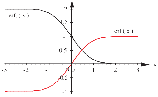
Refer to caption
Figure 10: Plot of erf(xx) and erfc(xx).

The Error Function is defined for real xx by

erf⁡(x)=2π​∫0xd​ξ​e−ξ2.{\rm erf}(x)=\frac{2}{\sqrt{\pi}}\int_{0}^{x}d\xi\;e^{-\xi^{2}}\;. (191)

erf⁡(x){\rm erf}(x) can be analytically continued to complex xx, but we have no need to consider such an extension in this paper. The complement of the Error Function is defined by

erfc⁡(x)=1−erf⁡(x)=2π​∫x∞d​ξ​e−ξ2.{\rm erfc}(x)=1-{\rm erf}(x)=\frac{2}{\sqrt{\pi}}\int_{x}^{\infty}d\xi\;e^{-\xi^{2}}\;. (192)

See Fig.10 for a plot of erf(xx) and erfc(xx). Under reflection x→−xx\rightarrow-x, erf(xx) obeys

erf⁡(−x)=−erf⁡(x),{\rm erf}(-x)=-{\rm erf}(x)\;, (193)

and erfc() obeys

erfc⁡(−x)=1−erf⁡(−x)=2−erfc⁡(x).{\rm erfc}(-x)=1-{\rm erf}(-x)=2-{\rm erfc}(x)\;. (194)

For real xx such that |x|<<1|x|<<1,

erf⁡(x)=2π​(x−x33⋅1!+x55⋅2!−x77⋅3!+…).{\rm erf}(x)=\frac{2}{\sqrt{\pi}}\left(x-\frac{x^{3}}{3\cdot 1!}+\frac{x^{5}}{5\cdot 2!}-\frac{x^{7}}{7\cdot 3!}+\ldots\right)\;. (195)

For real xx such that |x|>>1|x|>>1,

erfc⁡(x)=2​θ​(x<0)+e−x2x​π​(1−12​x2+1⋅3(2​x2)2−1⋅3⋅5(2​x2)3+…).{\rm erfc}(x)=2\theta(x<0)+\frac{e^{-x^{2}}}{x\sqrt{\pi}}\left(1-\frac{1}{2x^{2}}+\frac{1\cdot 3}{(2x^{2})^{2}}-\frac{1\cdot 3\cdot 5}{(2x^{2})^{3}}+\ldots\right)\;. (196)
Claim A.1

For a,b,Λ∈R​e​a​l​sa,b,{\Lambda}\in Reals with Λ,a>0{\Lambda},a>0,

erfc⁡(b2​a)=1π​i​∫Λ−i​∞Λ+i​∞d​λλ​exp⁡(a​λ2−b​λ).{\rm erfc}(\frac{b}{2\sqrt{a}})=\frac{1}{\pi i}\int_{{\Lambda}-i\infty}^{{\Lambda}+i\infty}\frac{d{\lambda}}{{\lambda}}\;\exp(a{\lambda}^{2}-b{\lambda})\;. (197)

proof:

erfc⁡(x)\displaystyle{\rm erfc}(x) =\displaystyle= 2π​∫−∞+∞d​ξ​e−ξ2​θ​(ξ>x)\displaystyle\frac{2}{\sqrt{\pi}}\int_{-\infty}^{+\infty}d\xi\;e^{-\xi^{2}}\theta(\xi>x) (198a)
=\displaystyle= 1π32​i​∫Λ−i​∞Λ+i​∞d​λλ​∫−∞+∞d​ξ​exp⁡(−ξ2+λ​ξ−λ​x)\displaystyle\frac{1}{\pi^{\frac{3}{2}}i}\int_{{\Lambda}-i\infty}^{{\Lambda}+i\infty}\frac{d{\lambda}}{{\lambda}}\int_{-\infty}^{+\infty}d\xi\;\exp(-\xi^{2}+{\lambda}\xi-{\lambda}x) (198b)
=\displaystyle= 1π​i​∫Λ−i​∞Λ+i​∞d​λλ​exp⁡(λ24−λ​x).\displaystyle\frac{1}{\pi i}\int_{{\Lambda}-i\infty}^{{\Lambda}+i\infty}\frac{d{\lambda}}{{\lambda}}\;\exp(\frac{{\lambda}^{2}}{4}-{\lambda}x)\;. (198c)

In Eq.(198), we went from line (a) to (b) by using the integral representation of the theta function, as given by Eq.(20). Now make the replacements λ→2​a​λ{\lambda}\rightarrow 2\sqrt{a}{\lambda}, x→b2​ax\rightarrow\frac{b}{2\sqrt{a}} in Eq.(198c). QED

Appendix B Appendix: Taylor Expansions Related to Information Theory

This handy appendix collects in one place several Taylor expansions that arise frequently in Information Theory.

For real xx such that |x|<1|x|<1,

ln⁡(1+x)\displaystyle\ln(1+x) =\displaystyle= ∑n=1∞(−1)n+1​xnn\displaystyle\sum_{n=1}^{\infty}\frac{(-1)^{n+1}x^{n}}{n} (199a)
=\displaystyle= x−x22+x33+….\displaystyle x-\frac{x^{2}}{2}+\frac{x^{3}}{3}+\ldots\;. (199b)

Thus, for |hx|<1|\frac{h}{x}|<1,

ln⁡(x+h)\displaystyle\ln(x+h) =\displaystyle= ln⁡[x⁡(1+hx)]=ln⁡x+∑n=1∞(−1)n+1​(hx)nn\displaystyle\ln[x(1+\frac{h}{x})]=\ln x+\sum_{n=1}^{\infty}\frac{(-1)^{n+1}(\frac{h}{x})^{n}}{n} (200a)
=\displaystyle= ln⁡x+hx−h22​x2+…,\displaystyle\ln x+\frac{h}{x}-\frac{h^{2}}{2x^{2}}+\ldots\;, (200b)
(x+h)​ln⁡(x+h)\displaystyle(x+h)\ln(x+h) =\displaystyle= x​ln⁡x+h⁡(ln⁡x+1)+h​∑n=2∞(−1)nn⁡(n−1)​(hx)n−1\displaystyle x\ln x+h(\ln x+1)+h\sum_{n=2}^{\infty}\frac{(-1)^{n}}{n(n-1)}\left(\frac{h}{x}\right)^{n-1} (201a)
=\displaystyle= x​ln⁡x+h⁡(ln⁡x+1)+h22​x+….\displaystyle x\ln x+h(\ln x+1)+\frac{h^{2}}{2x}+\ldots\;. (201b)

Let Δ​P​(x)=P⁡(x)−Q⁡(x)\Delta P(x)=P(x)-Q(x). Then

H⁡(P)\displaystyle H(P) =\displaystyle= −∑xP(x)lnP(x)\displaystyle-\sum_{x}P(x)\ln P(x) (202a)
=\displaystyle= H⁡(Q)−∑xΔ​P​(x)​ln⁡Q⁡(x)−∑x[Δ​P​(x)]22​Q​(x)+𝒪⁡((Δ​P)3),\displaystyle H(Q)-\sum_{x}\Delta P(x)\ln Q(x)-\sum_{x}\frac{[\Delta P(x)]^{2}}{2Q(x)}+{\cal O}((\Delta P)^{3})\;, (202b)

and

D(P//Q)\displaystyle D(P//Q) =\displaystyle= ∑xP⁡(x)​ln⁡P⁡(x)Q⁡(x)\displaystyle\sum_{x}P(x)\ln\frac{P(x)}{Q(x)} (203a)
=\displaystyle= ∑x[Δ​P​(x)]22​Q​(x)+𝒪⁡((Δ​P)3).\displaystyle\sum_{x}\frac{[\Delta P(x)]^{2}}{2Q(x)}+{\cal O}((\Delta P)^{3})\;. (203b)

Appendix C Appendix: Gaussian Integration Formulae

In this appendix, we present certain integration formulae that contain a Gaussian times a delta or a theta function in the integrand.

The following lemma will be used to prove Claim C.1, which is the main result of this appendix.

Lemma C.1

Suppose A∈R​e​a​l​sn×nA\in Reals^{n\times n} is invertible, v∈R​e​a​l​sn×1v\in Reals^{n\times 1}, vT​A−1​v≠0v^{T}A^{-1}v\neq 0, 0<ϵ<<10<\epsilon<<1, and

B=A+v​vTϵ.B=A+\frac{vv^{T}}{\epsilon}\;. (204)

Then the inverse and determinant of B are given by

B−1=A−1−A−1​A~​A−1​where​A~=v​vTvT​A−1​v,B^{-1}=A^{-1}-A^{-1}\tilde{A}A^{-1}\;\;{\rm where}\;\;\tilde{A}=\frac{vv^{T}}{v^{T}A^{-1}v}\;, (205)

and

detB=det(A)​vT​A−1​vϵ.\det B=\det(A)\frac{v^{T}A^{-1}v}{\epsilon}\;. (206)

proof:

It is easy to show that if uu and vv are nn dimensional column vectors and

B=A+u​vT,B=A+uv^{T}\;, (207)

then

B−1=A−1−A−1​u​vT​A−11+vT​A−1​uB^{-1}=A^{-1}-\frac{A^{-1}uv^{T}A^{-1}}{1+v^{T}A^{-1}u}\; (208)

satisfies B​B−1=B−1​B=1BB^{-1}=B^{-1}B=1. Setting u=v/ϵu=v/\epsilon and taking the limit ϵ→0\epsilon\rightarrow 0 yields Eq.(205).

To show Eq.(206), recall that

ln⁡(detA)=tr⁡(ln⁡A).\ln(\det A)={\rm tr}(\ln A)\;. (209)

(This well known identity is obvious when AA is diagonal. The proof is also very simple when AA is non-diagonal but diagonalizable.) If the entries of AA are taken to be independent variables, then Eq.(209) implies

δ​ln⁡(detA)=tr⁡(A−1​δ​A)=∑i,j(A−1)i​j​δ​Aj​i.\delta\ln(\det A)={\rm tr}(A^{-1}\delta A)=\sum_{i,j}(A^{-1})_{ij}\delta A_{ji}\;. (210)

Therefore,

(A−1)i​j=∂∂Aj​i​ln​detA=1detA​∂(detA)∂Aj​i.(A^{-1})_{ij}=\frac{\partial}{\partial A_{ji}}\ln\det A=\frac{1}{\det A}\frac{\partial(\det A)}{\partial A_{ji}}\;. (211)

This is just the usual expansion of A−1A^{-1} in terms of cofactors. For definiteness, suppose AA is a 3×33\times 3 matrix with columns a1→,a2→,a3→\vec{a_{1}},\vec{a_{2}},\vec{a_{3}}. Suppose uu and vv are also 3×13\times 1 column vectors. Then

det(A+u​vT)=det[a→1+v1​u→,a→2+v2​u→,a→2+v3​u→]\displaystyle\det(A+uv^{T})=\det[\vec{a}_{1}+v^{1}\vec{u},\vec{a}_{2}+v^{2}\vec{u},\vec{a}_{2}+v^{3}\vec{u}] (212a)
=\displaystyle= detA+det[v1​u→,a→2,a→3]+det[a→1,v2​u→,a→3]+det[a→1,a→2,v3​u→]\displaystyle\det A+\det[v^{1}\vec{u},\vec{a}_{2},\vec{a}_{3}]+\det[\vec{a}_{1},v^{2}\vec{u},\vec{a}_{3}]+\det[\vec{a}_{1},\vec{a}_{2},v^{3}\vec{u}] (212b)
=\displaystyle= det(A)+∑i,juj​∂(detA)∂Aj​i​vi\displaystyle\det(A)+\sum_{i,j}u^{j}\;\frac{\partial(\det A)}{\partial A_{ji}}\;v^{i} (212c)
=\displaystyle= det(A)​(1+vT​A−1​u).\displaystyle\det(A)(1+v^{T}A^{-1}u)\;. (212d)

In Eq.(212), we went from line (a) to (b) by using the fact that determinants are linear functions of each column. We also used the fact that determinants with a pair of proportional columns are zero, so that, for example,

det[v1​u→,v2​u→,a→3]=0.\det[v^{1}\vec{u},v^{2}\vec{u},\vec{a}_{3}]=0\;. (213)

Now setting u=v/ϵu=v/\epsilon in Eq.(212) yields

det(B)\displaystyle\det(B) =\displaystyle= det(A)​(1+vT​A−1​vϵ)\displaystyle\det(A)\left(1+\frac{v^{T}A^{-1}v}{\epsilon}\right) (214a)
≈\displaystyle\approx det(A)​(vT​A−1​vϵ).\displaystyle\det(A)\left(\frac{v^{T}A^{-1}v}{\epsilon}\right)\;. (214b)

QED

Claim C.1

For x,b∈R​e​a​l​sN×1x,b\in Reals^{N\times 1} and A∈R​e​a​l​sN×NA\in Reals^{N\times N}, define a measure d​G​(x)dG(x) so that for any real valued function f⁡(x)f(x),

∫d​G​(x)​f​(x)=∏{∫−∞+∞d​xj}∀j∈Z1,N​exp⁡(−xT​A​x2+bT​x)​f​(x).\int dG(x)\;f(x)=\prod\left\{{\int_{-\infty}^{+\infty}dx_{j}}\right\}_{\forall j\in Z_{1,N}}\exp\left(\frac{-x^{T}Ax}{2}+b^{T}x\right)f(x)\;. (215)

Suppose AA is a real, positive definite, symmetric matrix. Suppose u,v∈R​e​a​l​sN×1u,v\in Reals^{N\times 1} and α∈R​e​a​l​s\alpha\in Reals. Define

A~=v​vTvT​A−1​v,B−1=A−1−A−1​A~​A−1.\tilde{A}=\frac{vv^{T}}{v^{T}A^{-1}v}\;\;,\;\;B^{-1}=A^{-1}-A^{-1}\tilde{A}A^{-1}\;. (216)

Then

∫d​G​(x)​ 1=(2​π)N2detA​exp⁡(bT​A−1​b2),\int dG(x)\;1=\frac{{(2\pi)}^{\frac{N}{2}}}{\sqrt{\det A}}\exp\left(\frac{b^{T}A^{-1}b}{2}\right)\;, (217a)
∫d​G​(x)​δ​(vT​x)=[∫d​G​(x)​ 1]​12​π​vT​A−1​v​exp⁡(−bT​A−1​A~​A−1​b2),\int dG(x)\;\delta(v^{T}x)=[\int dG(x)\;1]\frac{1}{\sqrt{2\pi v^{T}A^{-1}v}}\exp\left(\frac{-b^{T}A^{-1}\tilde{A}A^{-1}b}{2}\right)\;, (217b)
∫d​G​(x)​θ​(uT​x−α≥0)=[∫d​G​(x)​ 1]​12​erfc​[α−uT​A−1​b2​uT​A−1​u],\int dG(x)\;\theta(u^{T}x-\alpha\geq 0)=[\int dG(x)\;1]\frac{1}{2}{\rm erfc}\left[\frac{\alpha-u^{T}A^{-1}b}{\sqrt{2u^{T}A^{-1}u}}\right]\;, (217c)
∫d​G​(x)​δ​(vT​x)​θ​(uT​x−α≥0)=[∫d​G​(x)​δ​(vT​x)]​12​erfc​[α−uT​B−1​b2​uT​B−1​u].\int dG(x)\;\delta(v^{T}x)\theta(u^{T}x-\alpha\geq 0)=[\int dG(x)\;\delta(v^{T}x)]\frac{1}{2}{\rm erfc}\left[\frac{\alpha-u^{T}B^{-1}b}{\sqrt{2u^{T}B^{-1}u}}\right]\;. (217d)

proof of Eq.(217a) :

Since AA is symmetric, it can be diagonalized. By diagonalizing AA, one can convert ∫d​G​(x)​1\int dG(x)1 into a product of one dimensional Gaussian integrals.

proof of Eq.(217b) :

For 0<ϵ<<10<\epsilon<<1,

δ⁡(vT​x)≈12​π​ϵ​exp⁡(−(vT​x)22​ϵ).\delta(v^{T}x)\approx\frac{1}{\sqrt{2\pi\epsilon}}\exp\left(\frac{-(v^{T}x)^{2}}{2\epsilon}\right)\;. (218)

Define BB by

B=A+vT​vϵ.B=A+\frac{v^{T}v}{\epsilon}\;. (219)

Then

∫d​G​(x)​δ​(vT​x)\displaystyle\int dG(x)\;\delta(v^{T}x) =\displaystyle= 12​π​ϵ​∏{∫−∞+∞d​xj}∀j∈Z1,N​exp⁡(−xT​B​x2+bT​x)\displaystyle\frac{1}{\sqrt{2\pi\epsilon}}\prod\left\{{\int_{-\infty}^{+\infty}dx_{j}}\right\}_{\forall j\in Z_{1,N}}\exp\left(\frac{-x^{T}Bx}{2}+b^{T}x\right) (220a)
=\displaystyle= 12​π​ϵ​(2​π)N2detB​exp⁡(bT​B−1​b2).\displaystyle\frac{1}{\sqrt{2\pi\epsilon}}\frac{{(2\pi)}^{\frac{N}{2}}}{\sqrt{\det B}}\exp\left(\frac{b^{T}B^{-1}b}{2}\right)\;. (220b)

Now use the values for B−1B^{-1} and detB\det B calculated in Lemma C.1.

proof of Eq.(217c) :

∫d​G​(x)​θ​(uT​x−α≥0)=∫d​G​(x)​12​π​i​∫Λ−i​∞Λ+i​∞d​λλ​eλ⁡(uT​x−α)\displaystyle\int dG(x)\;\theta(u^{T}x-\alpha\geq 0)=\int dG(x)\frac{1}{2\pi i}\int_{\Lambda-i\infty}^{\Lambda+i\infty}\frac{d{\lambda}}{{\lambda}}\;e^{{\lambda}(u^{T}x-\alpha)} (221a)
=\displaystyle= 12​π​i​∫Λ−i​∞Λ+i​∞d​λλ​∫d​xN​exp⁡(−xT​A​x2+(b+λ​u)T​x−λ​α)\displaystyle\frac{1}{2\pi i}\int_{\Lambda-i\infty}^{\Lambda+i\infty}\frac{d{\lambda}}{{\lambda}}\;\int dx^{N}\exp\left(\frac{-x^{T}Ax}{2}+(b+{\lambda}u)^{T}x-{\lambda}\alpha\right) (221b)
=\displaystyle= 12​π​i​∫Λ−i​∞Λ+i​∞d​λλ​(2​π)N2detA​exp⁡((b+λ​u)T​A−1​(b+λ​u)2−λ​α)\displaystyle\frac{1}{2\pi i}\int_{\Lambda-i\infty}^{\Lambda+i\infty}\frac{d{\lambda}}{{\lambda}}\;\frac{{(2\pi)}^{\frac{N}{2}}}{\sqrt{\det A}}\exp\left(\frac{(b+{\lambda}u)^{T}A^{-1}(b+{\lambda}u)}{2}-{\lambda}\alpha\right) (221d)
=\displaystyle= 12​π​i​(2​π)N2detA​exp⁡(bT​A−1​b2)\displaystyle\frac{1}{2\pi i}\frac{{(2\pi)}^{\frac{N}{2}}}{\sqrt{\det A}}\exp\left(\frac{b^{T}A^{-1}b}{2}\right)
∫Λ−i​∞Λ+i​∞d​λλ​exp⁡(λ2​(uT​A−1​u2)+λ⁡(uT​A−1​b−α))\displaystyle\int_{\Lambda-i\infty}^{\Lambda+i\infty}\frac{d{\lambda}}{{\lambda}}\;\exp\left({\lambda}^{2}(\frac{u^{T}A^{-1}u}{2})+{\lambda}(u^{T}A^{-1}b-\alpha)\right)
=\displaystyle= [∫d​G​(x)​ 1]​12​erfc​[α−uT​A−1​b2​uT​A−1​u].\displaystyle[\int dG(x)\;1]\frac{1}{2}{\rm erfc}\left[\frac{\alpha-u^{T}A^{-1}b}{\sqrt{2u^{T}A^{-1}u}}\right]\;. (221e)

In Eq.(221), line (a), we used the integral representation of the theta function given by Eq.(20). In Eq.(221), we went from line (b) to (c) by applying Eq.(217a). We went from line (d) to (e) by applying Eq.(197).

proof of Eq.(217d) :

This proof is similar to that of Eqs.(220) (a), (b) and (c) so it is left to the reader. QED

Appendix D Appendix: An Integral Over All
Joint Probability Distributions
with a Fixed Marginal

In this appendix, we will show how to convert (1) to (2) where (1) is an integral over all joint probability distributions Px¯,y¯P_{{\underline{x}},{\underline{y}}} with the same marginal Py¯P_{\underline{y}}, and (2) is an integral over all conditional probability distributions Px¯|y¯P_{{\underline{x}}|{\underline{y}}}.

Claim D.1
∫𝒟​Px¯,y¯​∏{δ⁡(P⁡(y)−Q⁡(y))}∀y​θ​(Px¯,y¯≥0)​f​(Px¯,y¯)=\displaystyle\int{\cal D}P_{{\underline{x}},{\underline{y}}}\;\prod\left\{{\delta(P(y)-Q(y))}\right\}_{\forall y}\theta(P_{{\underline{x}},{\underline{y}}}\geq 0)f(P_{{\underline{x}},{\underline{y}}})= (222)
∏{[Q⁡(y)]Nx¯−1}∀y​∫∏{d​P​(x|y)}∀x,y\displaystyle\prod\left\{{[Q(y)]^{N_{\underline{x}}-1}}\right\}_{\forall y}\int\prod\left\{{dP(x|y)}\right\}_{\forall x,y}
∏{δ⁡(∑xP⁡(x|y)−1)}∀y​θ​(Px¯|y¯≥0)​f​(Px¯,y¯).\displaystyle\prod\left\{{\delta(\sum_{x}P(x|y)-1)}\right\}_{\forall y}\theta(P_{{\underline{x}}|{\underline{y}}}\geq 0)f(P_{{\underline{x}},{\underline{y}}})\;.

proof:

Let RHS (ditto, LHS) stand for the right (ditto, left) hand side of Eq.(222). Suppose 0∈Sx¯0\in S_{\underline{x}}. Then

L​H​S\displaystyle LHS =\displaystyle= ∫∏⁡{d​P​(x,y)}∀(x,y),x≠0\displaystyle\int\prod\left\{{dP(x,y)}\right\}_{\forall(x,y),x\neq 0} (223b)
∏{θ[0≤∑x:x≠0P(x,y)≤Q(y)]}∀yθ(Px¯,y¯>0)f(P)\displaystyle\prod\left\{{\theta[0\leq\sum_{x:\;x\neq 0}P(x,y)\leq Q(y)]}\right\}_{\forall y}\theta(P_{{\underline{x}},{\underline{y}}}>0)f(P)
=\displaystyle= ∏{[Q⁡(y)]Nx¯−1}∀y​∫∏{d​P​(x|y)}∀(x,y),x≠0\displaystyle\prod\left\{{[Q(y)]^{N_{\underline{x}}-1}}\right\}_{\forall y}\int\prod\left\{{dP(x|y)}\right\}_{\forall(x,y),x\neq 0}
∏{θ(0≤∑x:x≠0P(x|y)≤1)}∀yθ(Px¯|y¯≥0)f(P)\displaystyle\prod\left\{{\theta(0\leq\sum_{x:\;x\neq 0}P(x|y)\leq 1)}\right\}_{\forall y}\theta(P_{{\underline{x}}|{\underline{y}}}\geq 0)f(P)
=\displaystyle= R​H​S.\displaystyle RHS\;. (223c)

QED

Appendix E Appendix: Perturbation Expansion of tt

In Eq.(156), we gave tt to lowest order in Δ​P\Delta P. In this appendix, we show how to calculate tt exactly, as a Taylor series in powers of Δ​P\Delta P.

The point P~∗{\tilde{P}}^{*} that dominates the integral Eq.(147) is an extremum of the Lagrangian Eq.(148). In Section 5.2, we approximated the Lagrangian Eq.(148) by its quadratic approximation Eq.(149). This gave us the dominant point P~∗{\tilde{P}}^{*} only to lowest order in Δ​P\Delta P. This time we will use the exact Lagrangian and get the exact dominant point. Let us re-state the exact Lagrangian:

ℒ=D(P~x¯,y¯//Qx¯,y¯)−λ(∑x,y(P−P~)(x,y)Lx​y)+∑yμy(P−P~)(y).{\cal L}=D({\tilde{P}}_{{\underline{x}},{\underline{y}}}//Q_{{\underline{x}},{\underline{y}}})-{\lambda}\left(\sum_{x,y}(P-{\tilde{P}})(x,y)L_{xy}\right)+\sum_{y}\mu_{y}(P-{\tilde{P}})(y)\;. (224)

Minimizing this Lagrangian with respect to P~{\tilde{P}}, λ{\lambda} and μy\mu_{y} gives

P~∗​(x,y)=Q⁡(x|y)​exp⁡(−λ​Lx​y)Zy​(λ)​P​(y),{\tilde{P}}^{*}(x,y)=\frac{Q(x|y)\exp(-{\lambda}L_{xy})}{Z_{y}({\lambda})}P(y)\;, (225)

where

Zy​(λ)=∑xQ⁡(x|y)​exp⁡(−λ​Lx​y).Z_{y}({\lambda})=\sum_{x}Q(x|y)\exp(-{\lambda}L_{xy})\;. (226)

The parameter λ{\lambda} in Eq.(225) is specified implicitly by the equation:

∑x,yP⁡(x,y)​Lx​y\displaystyle\sum_{x,y}P(x,y)L_{xy} =\displaystyle= ∑x,yQ⁡(x|y)​exp⁡(−λ​Lx​y)Zy​(λ)​P​(y)​Lx​y\displaystyle\sum_{x,y}\frac{Q(x|y)\exp(-{\lambda}L_{xy})}{Z_{y}({\lambda})}P(y)L_{xy} (227a)
=\displaystyle= −∑yP(y)d​ln⁡Zy​(λ)d​λ.\displaystyle-\sum_{y}P(y)\frac{d\ln Z_{y}({\lambda})}{d{\lambda}}\;. (227b)

The previous equation can be rewritten as

0=ϵ+F⁡(λ),0=\epsilon+F({\lambda})\;, (228)

where ϵ\epsilon and F⁡(λ)F({\lambda}) are defined by

ϵ=∑x,yP⁡(y)​Δ​P​(x|y)​Lx​y,\epsilon=\sum_{x,y}P(y)\Delta P(x|y)L_{xy}\;, (229)

and

F⁡(λ)=∑yP⁡(y)​[d​ln⁡Zy​(λ)d​λ−(d​ln⁡Zy​(λ)d​λ)λ=0].F({\lambda})=\sum_{y}P(y)\left[\frac{d\ln Z_{y}({\lambda})}{d{\lambda}}-\left(\frac{d\ln Z_{y}({\lambda})}{d{\lambda}}\right)_{{\lambda}=0}\right]\;. (230)

Next we will solve Eq.(228) for λ{\lambda} by expressing λ{\lambda} as a Taylor series in powers of ϵ\epsilon. We begin by expressing the RHS of Eq.(226) as a Taylor series in powers of λ{\lambda}:

Zy​(λ)=∑k=0∞Ak​(y)​(−λ)kk!,Z_{y}({\lambda})=\sum_{k=0}^{\infty}\frac{A_{k}(y)(-{\lambda})^{k}}{k!}\;, (231)

where

Ak​(y)=∑xQ⁡(x|y)​(Lx​y)kA_{k}(y)=\sum_{x}Q(x|y)(L_{xy})^{k}\; (232)

for k=0,1,2,⋯k=0,1,2,\cdots. It follows that

ln⁡Zy​(λ)=a1​λ+a2​λ22+a3​λ33+…,\ln Z_{y}({\lambda})=a_{1}{\lambda}+a_{2}\frac{{\lambda}^{2}}{2}+a_{3}\frac{{\lambda}^{3}}{3}+\ldots\;, (233)

where

a1=−A1,a_{1}=-A_{1}\;, (234a)
a2=−A12+A2,a_{2}=-A_{1}^{2}+A_{2}\;, (234b)
a3=−A13+32​A1​A2−12​A3,a_{3}=-A_{1}^{3}+\frac{3}{2}A_{1}A_{2}-\frac{1}{2}A_{3}\;, (234c)
a4=−A14+2​A2​A12−23​A1​A3−12​A22+16​A4.a_{4}=-A_{1}^{4}+2A_{2}A_{1}^{2}-\frac{2}{3}A_{1}A_{3}-\frac{1}{2}A_{2}^{2}+\frac{1}{6}A_{4}\;. (234d)

Define

αk=∑yP⁡(y)​ak​(y)\alpha_{k}=\sum_{y}P(y)a_{k}(y)\; (235)

for k=1,2,3,…k=1,2,3,\ldots. If we express F⁡(λ)F({\lambda}) as a Taylor series in powers of λ{\lambda}

F⁡(λ)=F1​λ+F2​λ2+F3​λ3+…,F({\lambda})=F_{1}{\lambda}+F_{2}{\lambda}^{2}+F_{3}{\lambda}^{3}+\ldots\;, (236)

then, by virtue of Eqs.(230), (233) and (235),

Fk=αk+1F_{k}=\alpha_{k+1}\; (237)

for k=1,2,3,…k=1,2,3,\ldots. Eq.(228) can be expressed as a Taylor series in powers of λ{\lambda}:

0=ϵ+F1​λ+F2​λ2+F3​λ3+….0=\epsilon+F_{1}{\lambda}+F_{2}{\lambda}^{2}+F_{3}{\lambda}^{3}+\ldots\;. (238)

λ{\lambda} itself can be expressed as a Taylor series in powers of ϵ\epsilon:

λ=λ1​ϵ+λ2​ϵ2+λ3​ϵ3+….{\lambda}={\lambda}_{1}\epsilon+{\lambda}_{2}\epsilon^{2}+{\lambda}_{3}\epsilon^{3}+\ldots\;. (239)

Substituting Eq.(239) into Eq.(238) yields an equation for each power of ϵ\epsilon. These equations for each power of ϵ\epsilon imply:

λ1=−1F1,{\lambda}_{1}=\frac{-1}{F_{1}}\;, (240a)
λ2=−F2F13,{\lambda}_{2}=\frac{-F_{2}}{F_{1}^{3}}\;, (240b)
λ3=F3​F1−2​F22F15,{\lambda}_{3}=\frac{F_{3}F_{1}-2F_{2}^{2}}{F_{1}^{5}}\;, (240c)
λ4=−5​F23+5​F3​F2​F1−F4​F12F17.{\lambda}_{4}=\frac{-5F_{2}^{3}+5F_{3}F_{2}F_{1}-F_{4}F_{1}^{2}}{F_{1}^{7}}\;. (240d)

Now that we know P~x¯,y¯∗{\tilde{P}}^{*}_{{\underline{x}},{\underline{y}}} explicitly (in terms of Eq.(225), where λ{\lambda} is expressed as a Taylor series in powers of ϵ\epsilon), we can find explicitly ℒ{\cal L} given by Eq.(224) evaluated at P~x¯,y¯∗{\tilde{P}}^{*}_{{\underline{x}},{\underline{y}}} .

ℒ∗\displaystyle{\cal L}^{*} =\displaystyle= D(P~y¯∗//Qy¯)+∑x,yP~∗(x,y)ln(P~∗​(x|y)Q⁡(x|y))\displaystyle D({\tilde{P}}^{*}_{\underline{y}}//Q_{\underline{y}})+\sum_{x,y}{\tilde{P}}^{*}(x,y)\ln\left(\frac{{\tilde{P}}^{*}(x|y)}{Q(x|y)}\right) (241a)
=\displaystyle= D(Py¯//Qy¯)+∑x,yP~∗(x,y)ln(exp⁡(−λ​Lx​y)Zy​(λ))\displaystyle D(P_{\underline{y}}//Q_{\underline{y}})+\sum_{x,y}{\tilde{P}}^{*}(x,y)\ln\left(\frac{\exp(-{\lambda}L_{xy})}{Z_{y}({\lambda})}\right) (241b)
=\displaystyle= D(Py¯//Qy¯)−λ∑x,yP(x,y)Lx​y−∑yP(y)lnZy(λ).\displaystyle D(P_{\underline{y}}//Q_{\underline{y}})-{\lambda}\sum_{x,y}P(x,y)L_{xy}-\sum_{y}P(y)\ln Z_{y}({\lambda})\;. (241c)

Expanding the ln⁡Zy​(λ)\ln Z_{y}({\lambda}) in the previous equations in powers of λ{\lambda} yields

ℒ∗\displaystyle{\cal L}^{*} =\displaystyle= D(Py¯//Qy¯)−λ∑x,yP(x,y)Lx​y\displaystyle D(P_{\underline{y}}//Q_{\underline{y}})-{\lambda}\sum_{x,y}P(x,y)L_{xy} (242a)
−(λ​α1+λ2​α22+λ3​α33+⋯)\displaystyle-({\lambda}\alpha_{1}+{\lambda}^{2}\frac{\alpha_{2}}{2}+{\lambda}^{3}\frac{\alpha_{3}}{3}+\cdots)
=\displaystyle= D(Py¯//Qy¯)−(λϵ+λ2α22+λ3α33+⋯).\displaystyle D(P_{\underline{y}}//Q_{\underline{y}})-({\lambda}\epsilon+{\lambda}^{2}\frac{\alpha_{2}}{2}+{\lambda}^{3}\frac{\alpha_{3}}{3}+\cdots)\;. (242b)

Expanding λ{\lambda} in the previous equation in powers of ϵ\epsilon yields

ℒ∗=D(Py¯//Qy¯)+t,{\cal L}^{*}=D(P_{\underline{y}}//Q_{\underline{y}})+t\;, (243)

where

t=t1​ϵ+t2​ϵ2+t3​ϵ3+⋯,t=t_{1}\epsilon+t_{2}\epsilon^{2}+t_{3}\epsilon^{3}+\cdots\;, (244)

and

t1=0,t_{1}=0\;, (245a)
t2=12​α2,t_{2}=\frac{1}{2\alpha_{2}}\;, (245b)
t3=α33​α23,t_{3}=\frac{\alpha_{3}}{3\alpha_{2}^{3}}\;, (245c)
t4=2​α32−α4​α24​α25.t_{4}=\frac{2\alpha_{3}^{2}-\alpha_{4}\alpha_{2}}{4\alpha_{2}^{5}}\;. (245d)

Now that we know tt to all orders in ϵ\epsilon, we can also find γ1\gamma_{1} to all orders in ϵ\epsilon. Recall from Section 5.3 that for any real valued function f⁡(s)f(s) of s≥0s\geq 0,

D​f=lims→0(−1γ0)​∂f∂s,Df=\lim_{s\rightarrow 0}\left(\frac{-1}{\gamma_{0}}\right)\frac{\partial f}{\partial s}\;, (246)

so that D​P(s)=Δ​PDP^{(s)}=\Delta P. When ff is the kkth power of ϵ\epsilon,

D​ϵk\displaystyle D\epsilon^{k} =\displaystyle= k​ϵk−1​∑x,y[Δ​P​(x,y)−Q⁡(x|y)​Δ​P​(y)]​Lx​y\displaystyle k\epsilon^{k-1}\sum_{x,y}[\Delta P(x,y)-Q(x|y)\Delta P(y)]L_{xy} (247a)
=\displaystyle= k​ϵk.\displaystyle k\epsilon^{k}\;. (247b)

From Eq.(244) one gets

D​t={t1​ϵ+t2​2​ϵ2+t3​3​ϵ3+…+ϵ​D​t1+ϵ2​D​t2+ϵ3​D​t3+….Dt=\left\{\begin{array}[]{l}t_{1}\epsilon+t_{2}2\epsilon^{2}+t_{3}3\epsilon^{3}+\ldots\\ +\epsilon Dt_{1}+\epsilon^{2}Dt_{2}+\epsilon^{3}Dt_{3}+\ldots\end{array}\right.\;. (248)

One can use Eqs.(245) to calculate D​tkDt_{k} in terms of {αk}∀k\{\alpha_{k}\}_{\forall k} and {D​αk}∀k\{D\alpha_{k}\}_{\forall k}. For example, D​t2=−12​α22​D​α2Dt_{2}=\frac{-1}{2\alpha^{2}_{2}}D\alpha_{2}. By Eq.(235),

D​αk=∑yΔ​P​(y)​ak​(y),D\alpha_{k}=\sum_{y}\Delta P(y)a_{k}(y)\;, (249)

for k=1,2,3,…k=1,2,3,\ldots. Once we know tt and D​tDt to all orders in ϵ\epsilon, we can use Eq.(177) to find γ1\gamma_{1} to all orders in ϵ\epsilon.

References

  • [1] Nigel Goldenfeld, Lectures on Phase Transitions and the Renormalization Group (1992, Perseus Books).
  • [2] T.M. Cover, J.A. Thomas, Elements of Information Theory (1991, John Wiley).
  • [3] R.E. Blahut, Principles and Practice of Information Theory (1987, Addison-Wesley)
  • [4] G.F. Carrier, M. Krook, C.E. Pearson, Functions of a Complex Variable (1966, MacGraw-Hill); N. Bleistein, R. A. Handelsman, Asymptotic Expansions of Integrals (1986, Dover).
  • [5] R. Fletcher, Practical Methods of Optimization (2000, John Wiley).
  • [6] An alternative method of getting a good trial value for Δ​R(sfin)\Delta R^{({s_{\rm fin}})} is as follows. Note that γ0​(P,Q)\gamma_{0}(P,Q) and γ1​(P,Q)\gamma_{1}(P,Q) both tend to 12\frac{1}{2} as P→QP\rightarrow Q. Thus, a good trial value for Δ​R(sfin)\Delta R^{({s_{\rm fin}})} is e−sfin2​Δ​Re^{\frac{-{s_{\rm fin}}}{2}}\Delta R. Plug this value of Δ​R(sfin)\Delta R^{({s_{\rm fin}})} into Δ​P​(X)=B⁡(X)​Δ​R(sfin)\Delta P(X)=B(X)\Delta R^{({s_{\rm fin}})} and check that it gives P(sfin)​(X)∈[0,1]P^{({s_{\rm fin}})}(X)\in[0,1] for all XX. If not, then continue halving the trial value of Δ​R(sfin)\Delta R^{({s_{\rm fin}})} until P(sfin)​(X)∈[0,1]P^{({s_{\rm fin}})}(X)\in[0,1] for all XX. This occurs eventually, assuming Q⁡(X)≠0Q(X)\neq 0 for all XX.
  • [7] M. Abramowitz, I.A. Stegun, Handbook of Mathematical Functions (1974, Dover).