On the practicality of time-optimal two-qubit Hamiltonian simulation
Abstract
What is the time-optimal way of using a set of control Hamiltonians to obtain a desired interaction? Vidal, Hammerer and Cirac [Phys. Rev. Lett. 88 (2002) 237902] have obtained a set of powerful results characterizing the time-optimal simulation of a two-qubit quantum gate using a fixed interaction Hamiltonian and fast local control over the individual qubits. How practically useful are these results? We prove that there are two-qubit Hamiltonians such that time-optimal simulation requires infinitely many steps of evolution, each infinitesimally small, and thus is physically impractical. A procedure is given to determine which two-qubit Hamiltonians have this property, and we show that almost all Hamiltonians do. Finally, we determine some bounds on the penalty that must be paid in the simulation time if the number of steps is fixed at a finite number, and show that the cost in simulation time is not too great.
pacs
03.67.-a,03.67.LxI Introduction
A central question of quantum information science is to determine the minimal time required to perform a quantum computation using a set of physical resources known to be universal for computation. Our understanding of what resources are universal for computation is very well-developed, and it is known 11 1 See Dodd et al. 2002; Wocjan et al. 2002; Dür et al. 2001; Bennett et al. 2001; Nielsen et al. 2002; Vidal and Cirac 2001; Brylinski and Brylinski 2002; Bremner et al. 2002 and references therein; see also Jones and Knill 1999; Leung et al. 2000 for related work. that when fast local control is available, any unitary dynamics capable of generating entanglement is universal for computation. However, the question of using these resources in a time-optimal fashion is, by comparison, understood relatively poorly.
This paper considers a particular simplified setting, that of time-optimal simulation of two-qubit unitaries using a fixed interaction Hamiltonian and arbitrary fast local control. Arbitrary fast local control means that the evolution of the interaction Hamiltonian may be interrupted by arbitrary single-qubit operations, and that these operations take no time to perform. This assumption corresponds to certain experimental setups where single-qubit operations are performed on a much faster time scale than joint operations. Hammerer, Vidal and Cirac Hammerer et al. 2002; Vidal et al. 2002 have given a construction for this simulation, as well as an elegant expression for the minimum achievable simulation time.
The simulation scheme of Hammerer et al. uses, in general, an infinite number of steps to achieve time optimality. That is, the interaction Hamiltonian is, in general, interrupted an infinite number of times by local operations, and the time between each interruption is infinitesimal. A simulation scheme requiring infinitely many time steps is not practical for at least two reasons. First, the original premise that local operations can be performed in zero time is no longer valid if one must perform infinitely many of them. Second, the effects of noise on such a simulation will overwhelm the intended coherent dynamics. The purpose of our paper is to ask, first, whether infinitely many time steps are actually required, in general, for time-optimal simulation? We will find that the answer is yes. Indeed, we will show that the overwhelming majority of two-qubit interaction Hamiltonians have this property. Given this, we then address the question of determining how close to time optimal a simulation can get, given that one demands a simulation using only a finite number of time steps.
The paper is structured as follows. In Sec. II we review results about two-qubit time-optimal simulation in the limit of fast control. In Sec. III we provide a procedure for determining which two-qubit Hamiltonians require infinitesimal time steps when used in this setting. Finally, in Sec. IV we quantify the sacrifice that must be made to time-optimality when one insists on having a simulation using a finite number of time steps. Sec. V concludes the paper.
II Preliminaries
The purpose of this section is to introduce notation and to review some concepts and results associated with time-optimal two-qubit simulation in the limit of fast local control. We end the section with an introduction to the idea of a “lazy” two-qubit Hamiltonian.
II.1 Notation
Up to rescaling of the ground state energy, an arbitrary two-qubit Hamiltonian can be parameterised as follows:
| (1) |
where and are real 3-vectors, is a 3 by 3 real matrix, and is the vector of Pauli operators. With respect to the computational basis , the Pauli operators are represented by the following matrices:
| (2) |
When all the entries are zero we say that the Hamiltonian is local. Otherwise we say that the Hamiltonian is nonlocal. We say that a unitary is local if it can be expressed as a tensor product of single-qubit unitaries. Otherwise we say the unitary is nonlocal. We shall henceforth restrict the single-qubit unitaries to be elements of the special unitary group (i.e., the group of two-by-two unitaries having unit determinant).
II.2 Time optimal simulation
A simulation scheme to approximate an arbitrary two-qubit unitary, , using a fixed Hamiltonian, , and arbitrary local unitaries may, without loss of generality, be written as follows.
| (3) | |||||
where the parameters are nonnegative. That is, in order to achieve the desired dynamics we can apply as many times as we wish for arbitrary lengths of time, interspersed with arbitrary operations on the individual qubits. We occasionally refer to Eq. (3) as being a circuit for . It is worth noting that the assumption that contains no term and that single-qubit unitaries are in , implies that is in . These restrictions entail no loss in generality, as they simply take advantage of the fact that the global phase of a unitary operator is irrelevant.
Corresponding to the simulation Eq. (3) is the interaction time, which we define to be the total time for which the interaction Hamiltonian is applied. For a given and , there are many possible circuits each giving rise to a simulation of . Over this range of possible circuits for , there is a corresponding range of values for the interaction time. A circuit which achieves the minimum interaction time for a given and is said to be time-optimal. We define to be the minimum achievable interaction time for simulating using . Reference Hammerer et al. 2002 gives a simple expression for , in the two-qubit scenario. To discuss this result, we first briefly review the canonical form of a two-qubit unitary and two-qubit Hamiltonian operator.
II.3 The canonical form of and
For any unitary there exists a canonical decomposition Khaneja et al. 2001; Kraus and Cirac 2001,
| (4) |
where , , , and are single-qubit special unitaries, and , , and are unique real numbers satisfying
| (5) |
Although 15 parameters are needed in order to completely specify an arbitrary two-qubit unitary , the canonical decomposition shows us that the nonlocal behaviour of can be characterised in terms of only three parameters, , and . We call these three parameters the canonical-form parameters of and the operator the canonical form of .
The local parts ,,, and of the canonical decomposition do not affect the interaction time, as they can be trivially included in the first and last steps, and , of a simulation. Therefore the canonical-form parameters are all we need to know about in order to calculate the minimum required interaction time for Eq. (3).
How does one calculate the canonical-form parameters? For completeness, we review the method given in Appendix A of Hammerer et al. 2002.
In the following it will be helpful to take advantage of properties of the so-called magic basis Hill and Wootters 1997,
It is known Hill and Wootters 1997 that, when expressed in the magic basis, local two-qubit special unitaries are real, and canonical-form unitaries are diagonal. This means that in the magic basis the canonical decomposition looks like , where and are real orthogonal matrices, and is diagonal. The diagonal elements of can be easily written in terms of the canonical-form parameters of : if we define
| (6) |
then the diagonal elements of are , , , and . Note that Eq. (6) together with Eq. (5) implies that
| (7) |
We have that , so the eigenvalues of are just the squares of the diagonal elements of . That is,
| (8) |
To determine the canonical-form parameters for a particular , we first calculate the eigenvalues of (where the transpose is taken in the magic basis), then derive the via Eq. (8), and finally solve Eqs. (6). A word of caution: the task of deriving the from the is not as trivial as it may first seem. The problem is that, in general, there is no guarantee that the values will lie in any particular branch of the logarithm function. So, naively taking the argument of will not necessarily give you . A relatively simple procedure exists to correct for this problem Childs et al. 2003. However in the context of Sec. III we will see later that taking the logarithm of along the standard branch of the logarithm function will suffice to evaluate .
Closely related to the canonical form for a two-qubit unitary is the canonical form for a two-qubit Hamiltonian. It is discussed in section V.A of Bennett et al. 2002, where it is referred to as the normal form. Given the purely nonlocal part
| (9) |
of a Hamiltonian , when it is expressed in the form Eq. (1), the canonical form of is defined to be the unique Hermitian operator
| (10) |
that satisfies
| (11) |
for some local unitary , where . The existence and uniqueness of this canonical form is established in Bennett et al. 2002, where it is shown that , and are the singular values of the matrix , and .
The canonical form of a Hamiltonian encapsulates the nonlocal behaviour of the evolution of for very small time steps. This can be seen as follows. From sections III.B and V.A of Bennett et al. 2002 we can write
| (12) | |||||
for some local unitaries ,, , and . To order , the evolution of is given by a unitary having canonical-form parameters , and .
II.4 Expression for
We are almost ready to review the expression for given in Vidal et al. 2002; Hammerer et al. 2002. Before we do so we review the concept of special-majorization. Special-majorization describes a particular type of partial ordering of three-vectors. Its use in Vidal et al. 2002; Hammerer et al. 2002 allows certain results to be described very succinctly. To define special-majorization, it is necessary to first introduce the idea of a special-ordered three-vector. Given a real vector , the corresponding special-ordered vector is defined as follows. The absolute value of the components of are given by the absolute value of the components of rearranged in nonincreasing order. That is, for the permutation that gives . The definition is completed by specifying that and are nonnegative, and that has the same sign as the product . Then, is said to be special-majorized by (denoted ) if
| (13) | |||||
where and are the special-ordered versions of and .
Let be a two-qubit Hamiltonian having canonical form and let be a two-qubit unitary having canonical form . Then , the minimum time required to simulate using , is given by the minimum value of such that either
| (15) | |||||
| (16) |
holds.
II.5 The lazy Hamiltonian
We now introduce the the central concept of a “lazy” Hamiltonian. For a given two-qubit Hamiltonian , we define a function as follows:
| (17) |
That is, is the minimum total time for which the Hamiltonian must be applied, when it is being used together with arbitrary local unitaries, to simulate its own action . Such a simulation would be of the form
| (18) | |||||
The trivial “simulation” having the single step has an interaction time of . Thus the minimum achievable interaction time will be no greater than :
| (19) |
Under what circumstances will be less than ? It turns out that this question is very closely linked to our main question: what are the circumstances under which a time-optimal simulation will require infinitesimal time steps?
Consider the class of two-qubit Hamiltonians having the following property:
| (20) |
We shall say that a Hamiltonian is “lazy” if it is nonlocal and satisfies Eq. (20).
Proposition 1
If a Hamiltonian is lazy, then the time-optimal simulation of any two-qubit nonlocal unitary using requires infinitely many time steps.
Proof: Suppose there exists a time-optimal simulation scheme, of the form of Eq. (3), for a nonlocal using a lazy Hamiltonian , where the number of time steps is finite. At least one of the must be nonzero, otherwise the simulation would be unable to produce nonlocal dynamics. For such a nonzero , consider the corresponding factor in the simulation. Since is lazy, there exists a simulation for having an interaction time less than . If we substitute such a simulation for back into the simulation for , then the new simulation for now has a lesser interaction time than it did before. However this contradicts the assumption that the original simulation was time optimal. Hence the premise that the original simulation had finite time steps is false. Thus we conclude that any lazy Hamiltonian will require infinitesimal time steps when used for the time-optimal simulation of any nonlocal two-qubit unitary .
To show that a particular is lazy, it is sufficient to show that for all in some interval for any positive . To see this, note that if there is a simulation for with interaction time , then clearly there exists a simulation for with interaction time , for any positive integer . Thus, implies that for all positive integers . So, if for all , then for all .
III General Procedure
Which two-qubit Hamiltonians are lazy? We have seen in the previous section (proposition 1) that lazy two-qubit Hamiltonians require infinitely many time steps if they are to be used for time-optimal control, and thus are impractical. In this section we provide a simple set of sufficient conditions for a Hamiltonian to be lazy, expressed in terms of the parameters of the Hamiltonian. The parameterisation in Eq. (1) is more general than it needs to be for this purpose. We can simplify matters by using the fact that a Hamiltonian is lazy if and only if is lazy, where and are any single-qubit unitaries. This is a consequence of the fact that has the same canonical form as . Thus, without loss of generality we choose to only consider Hamiltonians where the purely nonlocal part is in canonical form, that is
| (21) |
where .
Recall from subsection II.5 that we define a Hamiltonian to be lazy if over some interval . Suppose we could find a Taylor series expansion
| (22) |
for in the variable . Thus,
| (23) |
Then, because we can assume is small, the corresponding Hamiltonian is lazy if and only if the first nonzero item in the list , , , , … is negative. Our procedure involves finding expressions for the first few items in that list, in terms of the parameters , and of the Hamiltonian. We then find the conditions under which each expression will be negative. We find that in fact always, and so is the first term that may be negative. Accordingly, in the analysis that follows we consider the behaviour of up to order , so as to arrive at some nontrivial conditions for a Hamiltonian being lazy.
III.1 Procedure to find the Taylor coefficients of
We seek expressions for the Taylor coefficients of , namely, , , , and . The expression for involves the canonical-form parameters , and of the unitary . So we first try to find expressions for the canonical-form parameters , and of the unitary . From subsection II.3, the canonical-form parameters can be expressed in terms of parameters , …, , where
| (24) |
with the transpose taken in the magic basis. Thus,
| (25) |
where the vector of integers accounts for the ambiguity in taking the argument, and where the down-arrow sorts in decreasing order so that we are in agreement with the ordering of the in Eq. (7). However, since we are only interested in the behaviour over a small interval , it turns out we can take . This can be seen as follows. From the discussion at the end of subsection II.4, for small the canonical-form parameters of will be small. Thus, the parameters … will also be small. But this can only be the case when . (A more rigorous proof of this fact is easily deduced from the procedure for finding the canonical-form parameters described in Childs et al. 2003.) Thus,
| (26) |
for in some interval .
Now, it is possible to write
| (27) |
where is given by the Campbell-Baker-Hausdorf series (for a derivation see, for example, Wilcox 1967)
| (28) | |||||
where . Thus, for we can write
| (29) | |||||
| (30) |
From Theorem 1.10 of Kato 1982, a normal-valued operator function that can be expressed as a power series
| (31) |
has eigenvalues which are holomorphic functions of . Thus, the entries of the vector can be expressed as holomorphic functions of , and the components of are therefore continuous piecewise-holomorphic functions of , over some interval . Approximating to some order in will give the same order of approximation for :
| (32) |
Define to be the first three terms in the expansion of in Eq. (28). That is,
| (33) | |||||
Then, if we define
| (34) |
we have
| (35) |
We can find the first four Taylor coefficients of each component of in the following way. Each component of satisfies the characteristic equation
| (36) |
We can substitute a Taylor series for :
| (37) |
Since Eq. (37) must be true for a range of values of , then all coefficients in a Taylor series for must be zero. Finding expressions for the coefficients , and solving the equations , will give us the coefficients , ,…etc. Note that when we wish to find a particular term , we need only include terms in the expansion of in Eq. (37) to order .
How can we use the Taylor coefficients of to find the Taylor coefficients of ? Does the ordering operation in Eq. (35) present a difficulty? Not really. Say that we knew the Taylor series for each of the four functions ,…,. We would simply order these vector components with respect to the zero-order Taylor coefficients: . If it happened that none of the were equal, that is , then Eq. (35) would immediately imply that
| (38) |
for in some interval . That is, for small , is equal to up to order , where the components of are arranged so the zeroth Taylor coefficients are in decreasing order. In the special case where some of the zero-order coefficients are equal, then we break the tie by considering the first-order coefficients, and if those are equal we consider the next highest order and so-on. In what follows, we will use the ordering scheme as described in this paragraph, so that we may use Eq. (38) instead of Eq. (35).
III.2 Procedure to find the Taylor coefficients of the components of .
In this subsection we describe the calculation of the Taylor coefficients of the components of .
In the magic basis, the Hamiltonian, , in Eq. (21) reads
The components of in the magic basis are found with the aid of the computer algebra system Maple. This is straightforward in any of the standard computer algebra systems, and the specific form is both complex and not particularly illuminating, so we will not reproduce the components of here. Note that each component is a third-order polynomial in .
Next, we find expressions for . To find , we evaluate the expression in Eq. (37) using Maple, including terms in the series up to at least order . Then, is given by the coefficient of the term in this expression. Explicit expressions for will not be given here as they are rather lengthy and not illuminating. They are polynomials in the parameters of the Hamiltonian.
The next step is to solve the equations , , via Maple. The results are as follows.
- •
- •
Solving , , and provides no new information about the .
- •
Solving yields four solutions, one for each component in . We write them in nonincreasing order as follows:
(45) This gives .
- •
Solving gives . Thus, .
- •
Solving gives four solutions to , so long as we assume . Each of the four solutions for correspond to one of the four solutions to (which were substituted in turn). Thus, we are able to correctly associate each of the four solutions to a particular component of the ordered vector . For the sake of brevity we will not reproduce the expressions for . Rather, we just provide the resulting expressions for :
The special cases , and provide different (and rather more complicated) solutions for the compared with above. Arriving at the solution in these cases requires solving up to . We will not write out these results explicitly.
Thus we have
| (47) |
for in some interval . is given in Eq. (), except in the special cases noted above.
III.3 Conditions for laziness
From section II.C of Hammerer et al. 2002, the expression for takes a simpler form when we have . In this special case, is given by the minimum value of such that
| (48) |
where again is the vector of canonical-form parameters of and is the vector of canonical-form parameters of . This special case certainly holds for the canonical-form parameters of when is sufficiently small. In this case Eq. (48) is equivalent to
| (49) |
which is equivalent to
| (50) |
Thus,
| (51) |
Given Eq. (47), we have
| (52) |
for small , where is given by
| (53) |
It is clear that whenever , the Hamiltonian is lazy. It is also clear that is never greater than zero, because that would imply , a contradiction. We find below the solutions (in terms of the parameters of the Hamiltonian) for ; all Hamiltonians which do not belong to this solution set are guaranteed to be lazy. Note, however, that the complement of this solution set does not entirely characterise the class of lazy Hamiltonians, since there may be Hamiltonians in this set that are lazy due to higher-order Taylor coefficients that are negative. So our results may not fully characterise the set of all lazy Hamiltonians.
Let
| (54) | |||||
| (55) | |||||
| (56) |
The coefficient is zero if and only if at least one of are zero. It is straightforward to show that for ,
| (57) | |||||
| (58) | |||||
| (59) |
We have arrived at the main result of this paper:
Result 1
Any Hamiltonian of the form of Eq. (21) for which and for which none of the three conditions
- 1.
- 2.
- 3.
hold, is lazy. Such Hamiltonians will therefore need to be applied infinitely many times when used in a time-optimal simulation of a nonlocal two-qubit unitary.
These conditions obviously make it very easy to generate examples of lazy Hamiltonians, and imply that almost all two-qubit Hamiltonians are lazy. Note that the special cases , and yield somewhat more complicated conditions for a Hamiltonian to be lazy. These conditions are complex and not very illuminating, but can be obtained using techniques similar to those described above, so we will not reproduce them here.
IV Using lazy Hamiltonian in finite time steps
The results of the previous section show that almost all two-qubit Hamiltonians are lazy. This means that, in a simulation circuit, infinitesimal time steps must be employed to achieve time-optimality. We now show that, despite this requirement, if finite time steps are used then the corresponding sacrifice of interaction time is not very large — only a small relaxation from strict time-optimality is required in order to reduce the number of time steps to something practical.
To make our results concrete, we consider the case where the unitary being simulated is the controlled-not (cnot) gate. Similar conclusions can be reached in the general case by following a similar argument to that below, and making use of the results of Zhang et al. 2002. It can be shown Hammerer et al. 2002 that the minimum time for simulating a cnot is where is the largest canonical-form parameter of the interaction Hamiltonian. When is lazy, can we construct a simulation using a finite number of time steps such that the total interaction time is not much larger than the optimum ? Such a scheme is given in Bremner et al. 2002, whereby an arbitrary nonlocal two-qubit unitary is applied a finite number of times together with local unitaries to simulate a cnot. Using the scheme in Bremner et al. 2002, if has largest canonical-form parameter such that
| (60) |
is an integer greater than one, then the scheme can be used to simulate a cnot by applying exactly times. Of course, we are interested in the case when , that is is given by the evolution of an interaction Hamiltonian over a time . The total interaction time would then be
| (61) |
From the previous section, the function can be written, for small , as
| (62) |
Thus, for small ,
| (63) | |||||
| (64) |
This shows that to simulate a cnot gate by applying a lazy interaction Hamiltonian in a (finite) number of small time-steps, then the penalty in the total interaction time, as compared with the optimum, is only of order .
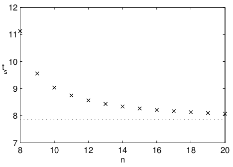
As an example, consider a specific interaction Hamiltonian . Using the results of the previous section it can easily be verified that is lazy. The graph of as a function of is shown in Fig. 1. We choose a range of positive integer values of , and for each we calculate how long the corresponding time step () is by numerically solving
| (65) |
No solution to Eq. (65) exists for . This can be seen from the fact that , which is greater than the maximum value that takes. For equal to 8 or greater, a corresponding can be found. Finally, the interaction time required to simulate the cnot is calculated via Eq. (61). The results are shown in Fig. 2. The dashed line is the optimal time, . The results clearly show a near-optimal simulation with relatively small numbers of time steps. For 20 time steps, the total interaction time is just percent greater than the optimal.

V Conclusions
We have defined a class of “lazy” two-qubit Hamiltonians, those which can simulate themselves faster with the aid of fast local control than with uninterrupted evolution. When a lazy Hamiltonian is used in the time-optimal simulation of any nonlocal two-qubit unitary, we have shown that the simulation will require an infinite number of steps, and thus will be impractical. We have derived a simple set of sufficient conditions enabling us to prove that a given Hamiltonian is lazy. This set of conditions implies that almost all two-qubit Hamiltonians are lazy. Finally, we have shown that only a rather small sacrifice in the simulation time needs to be made in order to use a lazy Hamiltonian in a finite-step simulation.
Acknowledgements.
Thanks to Chris Dawson for helpful discussions and for suggesting the name “lazy” Hamiltonian. Thanks also to Guifré Vidal for enlightening discussions. HLH and MAN enjoyed the hospitality of the Institute for Quantum Information at the California Institute of Technology, where part of this work was completed.References
- Hammerer et al. (2002) K. Hammerer, G. Vidal, and J. I. Cirac, Phys. Rev. A 66, 062321 (2002), arXiv:quant-ph/0205100.
- Vidal et al. (2002) G. Vidal, K. Hammerer, and J. I. Cirac, Phys. Rev. Lett. 88, 237902 (2002), arXiv:quant-ph/0112168.
- Khaneja et al. (2001) N. Khaneja, R. Brockett, and S. J. Glaser, Phys. Rev. A 65, 032308 (2001), arXiv:quant-ph/0006114.
- Kraus and Cirac (2001) B. Kraus and J. I. Cirac, Phys. Rev. A 53, 062309 (2001), arXiv:quant-ph/0011050.
- Hill and Wootters (1997) S. Hill and W. K. Wootters, Phys. Rev. Lett. 78, 5022 (1997), arXiv:quant-ph/9703041.
- Childs et al. (2003) A. M. Childs, H. L. Haselgrove, and M. A. Nielsen, In preparation (2003).
- Bennett et al. (2002) C. H. Bennett, J. I. Cirac, M. S. Leifer, D. W. Leung, N. Linden, S. Popescu, and G. Vidal, Phys. Rev. A 66, 012305 (2002), arXiv:quant-ph/0107035v2, updated version of Bennett et al. 2001.
- Wilcox (1967) R. M. Wilcox, J. Math. Phys. 8, 962 (1967).
- Kato (1982) T. Kato, A short introduction to perturbation theory for linear operators (Springer-Verlag, 1982).
- Zhang et al. (2002) J. Zhang, J. Vafa, S. Sastry, and K. B. Whaley, arXiv:quant-ph/0212109 (2002).
- Bremner et al. (2002) M. J. Bremner, C. M. Dawson, J. L. Dodd, A. Gilchrist, A. W. Harrow, D. Mortimer, M. A. Nielsen, and T. J. Osborne, Phys. Rev. Lett. 89, 247902 (2002), arXiv:quant-ph/0207072.
- Bennett et al. (2001) C. H. Bennett, J. I. Cirac, M. S. Leifer, D. W. Leung, N. Linden, S. Popescu, and G. Vidal, arXiv:quant-ph/0107035v1 (2001).
- Brylinski and Chen (2002) R. K. Brylinski and G. Chen, eds., Mathematics of Quantum Computation, Computational Mathematics (Chapman & Hall / CRC Press, 2002).
- Dodd et al. (2002) J. L. Dodd, M. A. Nielsen, M. J. Bremner, and R. T. Thew, Phys. Rev. A 65, 040301 (R) (2002), arXiv:quant-ph/0106064.
- Wocjan et al. (2002) P. Wocjan, D. Janzing, and T. Beth, Quantum Information and Computation 2, 117 (2002), arXiv:quant-ph/0106077.
- Dür et al. (2001) W. Dür, G. Vidal, J. I. Cirac, N. Linden, and S. Popescu, Phys. Rev. Lett. 87, 137901 (2001), arXiv:quant-ph/0006034v3 and later versions.
- Nielsen et al. (2002) M. A. Nielsen, M. J. Bremner, J. L. Dodd, A. M. Childs, and C. M. Dawson, Phys. Rev. A 66, 022317 (2002), arXiv:quant-ph/0109064.
- Vidal and Cirac (2001) G. Vidal and J. I. Cirac, arXiv:quant-ph/0108076 (2001).
- Brylinski and Brylinski (2002) J. L. Brylinski and R. Brylinski, Universal quantum gates (2002), chap. II in Brylinski and Chen 2002, arXiv:quant-ph/0108062.
- Jones and Knill (1999) J. A. Jones and E. Knill, Journal of Magnetic Resonance 141, 322 (1999).
- Leung et al. (2000) D. W. Leung, I. L. Chuang, F. Yamaguchi, and Y. Yamamoto, Phys. Rev. A 61, 042310 (2000).