The Quantum Four Stroke Heat Engine: Thermodynamic Observables in a Model with Intrinsic Friction

Tova Feldmann and Ronnie Kosloff Email: ronnie@fh.huji.ac.il Affiliation: Department of Physical Chemistry the Hebrew University, Jerusalem 91904, Israel

Abstract

The fundamentals of a quantum heat engine are derived from first principles. The study is based on the equation of motion of a minimum set of operators which is then used to define the state of the system. The relation between the quantum framework and thermodynamical observables is examined. A four stroke heat engine model with a coupled two-level-system as a working fluid is used to explore the fundamental relations. In the model used, the internal Hamiltonian does not commute with the external control field which defines the two adiabatic branches. Heat is transferred to the working fluid by coupling to hot and cold reservoirs under constant field values. Explicit quantum equation of motion for the relevant observables are derived on all branches. The dynamics on the heat transfer constant field branches is solved in closed form. On the adiabats, a general numerical solution is used and compared with a particular analytic solution. These solutions are combined to construct the cycle of operation. The engine is then analyzed in terms of frequency-entropy and entropy-temperature graphs. The irreversible nature of the engine is the result of finite heat transfer rates and friction-like behavior due to noncommutability of the internal and external Hamiltonian.

pacs

05.70.Ln, 07.20.Pe

I Introduction

Analysis of heat engine models has been a major part of thermodynamic development. For example Carnot’s engine preceded the concepts of energy and entropy carnot1824. Szilard and Brillouin constructed a model engine which enabled them to resolve the paradox raised by Maxwell’s demon szilard29; brillouin. The subsequent insight enabled the unification of negative entropy with information. In the same tradition, the present paper studies a heat engine model with a quantum working fluid for the purpose of tracing the microscopic origin of friction. The function of a quantum heat engine as well as its classical counterpart is to transform heat into useful work. In such engines, the work is extracted by an external field exploiting the spontaneous flow of heat from a hot to a cold reservoir. The present model performs this task by a four stroke cycle of operation. All four branches of the cycle can be described by quantum equations of motion. The thermodynamical consequences can therefore be derived from first principles.

The present paper lays the foundation for a comprehensive analysis of a discrete model of a quantum heat engine. A brief outline which has been published emphasized the engines optimal performance characteristics kosloff01. It was shown that the engines power output vs. cycle time mimics very closely a classical heat engine subject to friction. The source of the apparent friction was traced back to a quantum phenomena: the noncommutability of the external control field Hamiltonian and the internal Hamiltonian of the working medium.

The fundamental issue involved require a detailed and careful study. The approach followed is to derive the thermodynamical concepts from quantum principles. The connecting bridges are the quantum thermodynamical observables. Following the tradition of Gibbs a minimum set of observables is sought which are sufficient to characterize the performance of the engine. When the working fluid is in thermal equilibrium, the energy observable is sufficient to completely describe the state of the system and therefore all other observables. During the cycle of operation the working fluid is in a non-equilibrium state. In frictionless engines, where the internal Hamiltonian commutes with the external control field, the energy observable is still sufficient to characterize the engine’s cycle feldmann96; feldmann00. In the general case additional variables have to be added. For example in the current model, a set of three quantum thermodynamic observables is sufficient to characterize the performance. With only two additional variables the state of the working fluid can be characterized also . A knowledge of the state is necessary in order to evaluate the entropy and the dynamical temperature. These variables are crucial in establishing a thermodynamic perspective.

The current investigation is in line with previous studies of quantum heat engines kosloff01; feldmann96; feldmann00; lloyd; gustic; k24; geva0; geva1; geva2; chen02; bender00; bender02; gordon01; jose; geva02. All the studies of first principle quantum models have conformed to the laws of thermodynamics. These models have been either continuous resembling turbines geva2; gordon01; jose, or discrete as in the present model kosloff01; feldmann96; geva0; geva1; geva2. Surprisingly the performance characteristics of the models were in close resemblance to their realistic counterparts. Real heat engines operate far from the reversible conditions, where the maximum power is restricted due to finite heat transfer curzon75, internal friction and heat leaks benshaul79; salamon77; salamon80; gordon91; andresen83; bejan96; gordon98. Analysis of the quantum models of heat engines, based on a first principle dynamical theory, enable to pinpoint the fundamental origins of finite heat transfer, internal friction and heat leaks.

Studies of quantum continuous heat engine models have revealed most of the known characteristics of real engines. In accordance with finite time thermodynamics the power always exhibits a definite maximum salamon77, and the performance has been limited by heat leaks jose. Finally indications of restrictions due to friction like phenomena have been indicated geva2. The difficulty with the analysis is that it is very hard to separate the individual contributions in the case of a continuous operating engine.

To facilitate the interpretation a four stroke discrete engine has been chosen for analysis. The cycle of operation is controlled by the segments of time that the engine is in contact with a hot and cold bath and by the time interval required to vary the external field. To simplify the analysis the time segments where the working fluid is in contact with the heat baths are carried out at constant external field. Such a cycle of operation resembles the Otto cycle which is composed of two isochores where heat is transfered and two adiabats where work is done. This simplification allows to obtain the values of the thermodynamical observables during the cycle of operation from first principles in closed form.

II Quantum Thermodynamical observables and their dynamics

The quantum thermodynamical observables constitute a set of variables which are sufficient to completely describe the heat engine performance characteristics as well as the entropy and temperature changes of its working medium. The analysis of the performance requires a quantum dynamical description of the changes in the thermodynamical observables during the engine’s cycle of operation. The thermodynamical observables are associated with the expectation values of operators of the working medium. Using the formalism of von Neumann, an expectation of an observable $\langle{\bf\hat{A}}\rangle$ is defined by the scalar product between the operator ${\bf\hat{A}}$ representing the observable and the density operator ${{\boldsymbol{\mathrm{\hat{\rho}}}}}$ representing the state of the working medium:

\langle{\bf\hat{A}}\rangle~=~\left({\bf\hat{A}}\cdot{{{\boldsymbol{\mathrm{\rho}}}}}\right)~=~Tr\{{\bf\hat{A}}^{{\dagger}}~{{{\boldsymbol{\mathrm{\rho}}}}}\}~~~.

(1)

The dynamics of the working medium is subject to external change of variables as well as heat transport from the hot and cold reservoirs. The dynamics is then described within the formulation of quantum open systems lindblad76; alicki87, where the dynamics is generated by the Liouville super operator ${\cal L}$ either as an equation of motion for the state ${{{\boldsymbol{\mathrm{\rho}}}}}$ (Schrödinger picture):

\dot{{{{\boldsymbol{\mathrm{\rho}}}}}}~~=~~{\cal L}({{{\boldsymbol{\mathrm{\rho}}}}})~~~,

(2)

or as an equation of motion for the operator (Heisenberg picture):

\dot{\bf\hat{A}}~~=~~{\cal L}^{*}({\bf\hat{A}})~+~\frac{\partial{\bf\hat{A}}}{\partial t}~~~.

(3)

The second part of the r.h.s. appears since the operator ${\bf\hat{A}}$ can be explicitly time dependent.

Significant simplification is obtained lendi01 when:

•

a) The operators of interest form an orthogonal set ${\bf\hat{B}_{i}}$ i.e.

$\left({\bf\hat{B}_{i}}\cdot{\bf\hat{B}_{j}}\right)=\delta_{\bf ij}~~,$ (4)

where ${\bf\hat{B}_{0}}={\bf\hat{I}}$ is the identity operator.
•

b) The set is closed to the operation of ${\cal L}^{*}$ .

$\dot{\bf\hat{B}_{i}}~=~{\cal L}^{*}({\bf\hat{B}_{i}})=\sum_{\bf j}l_{\bf j}^{\bf i}{\bf\hat{B}_{j}}~~~,$ (5)

where $l_{\bf i}^{\bf j}$ are scalar coefficients composing the matrix $\tilde{L}$ .
•

c) The equilibrium density operator is a linear combination of the set:

${{{{\boldsymbol{\mathrm{\rho}}}}}}^{eq}~=~\frac{1}{N}{\bf\hat{I}}+\sum_{\bf k}b_{\bf k}^{eq}{\bf\hat{B}_{k}}~~~,$ (6)

where $N$ is the dimension of the Hilbert space and $b_{\bf k}^{eq}$ are the equilibrium expectation values of the the operators, $\langle{\bf\hat{B}_{k}}^{eq}\rangle$ .

The operator property of Eq. (5) allows a direct solution to the Heisenberg equation of motion (3) by diagonalizing the $\tilde{L}$ matrix, relating observables $\langle{\bf\hat{B}_{k}}\rangle$ at time $t$ to observables at time $t+\Delta t$ that is $\vec{\bf b}(t+\Delta t)={\cal U}(\Delta t)\vec{\bf b}(t)$ where ${\cal U}=e^{\tilde{L}\Delta t}$ and $\vec{\bf b}$ is a vector composed from the expectation values of ${\bf\hat{B}_{k}}$ ( for an example Cf. (III.2.1) ).

The time dependent expectation values $\vec{\bf b}(t)$ and Eq. (6) can be employed to reconstruct the density operator:

{{{{\boldsymbol{\mathrm{\rho}}}}}}_{R}~~=~~\frac{1}{N}{\bf\hat{I}}+\sum_{\bf k}b_{\bf k}{\bf\hat{B}_{k}}~~~,

(7)

where the expansion coefficients become $b_{\bf k}=\langle{\bf\hat{B}_{k}}\rangle$ . Although the set ${\bf\hat{B}_{k}}$ is not necessarily complete, equation (7) will still be used as a reconstructing method for the density operator. This reconstructed state ${{{{\boldsymbol{\mathrm{\rho}}}}}}_{R}$ reproduces all observations which are constructed from linear combinations of the set of operators ${\bf\hat{B}_{k}}$ .

The Liouville operator Eq. (2),(3) for an open quantum system can be partitioned into a unitary part ${\cal L}_{H}$ and a dissipative part ${\cal L}_{D}$ lindblad76:

{\cal L}={\cal L}_{H}+{\cal L}_{D}~~~.

(8)

The unitary part is generated by the Hamiltonian: $\bf\hat{H}$ :

{\cal L}_{H}^{*}({\bf\hat{A}})=i[{\bf\hat{H}},{\bf\hat{A}}]~~.

(9)

The condition for a set of operators to be closed under ${\cal L}_{H}^{*}$ have been well studied yoram. If the Hamiltonian can be decomposed to:

{\bf\hat{H}}=\sum_{\bf j}h_{\bf j}{\bf\hat{B}_{j}}~~~,

(10)

and the set ${\bf\hat{B}_{k}}$ forms a Lie algebra paldus88; wybourne i.e. $[{\bf\hat{B}_{i}},{\bf\hat{B}_{j}}]=\sum_{\bf k}C_{\bf ij}^{\bf k}{\bf\hat{B}_{k}}$ (the coefficients $C_{\bf ij}^{\bf k}$ are the structure factors of the Lie algebra), then the set is closed under ${\cal L}_{H}^{*}$ .

For the dissipative Liouville operator ${\cal L}_{D}$ , Lindblad’s form is used lindblad76:

\displaystyle{\cal L}_{D}^{*}(\bf\hat{A})~~=~~\Large\sum_{j}~\left({\bf\hat{F}}_{\rm j}{\bf\hat{A}}{\bf\hat{F}}_{\rm j}^{\dagger}-\frac{1}{2}(\bf\hat{F}_{\rm j}{\bf\hat{F}}_{\rm j}^{\dagger}{\bf\hat{A}}~+~{\bf\hat{A}}{\bf\hat{F}}_{\rm j}{\bf\hat{F}}_{\rm j}^{\dagger})\right)~~~,

(11)

where $\bf\hat{F}_{\rm j}$ are operators from the Hilbert space of the system. The conditions for which the set ${\bf\hat{B}}_{i}$ is closed to ${\cal L}_{D}^{*}$ have not been well established. Nevertheless in the present studied example such a set has been found.

II.1 Energy balance

The energy balance of the working medium is followed by the changes in time to the expectation value of the Hamiltonian operator. For a working medium composed of a gas of interacting particles the Hamiltonian is described as:

{\bf\hat{H}}~~=~~{\bf\hat{H}_{ext}}~+~{\bf\hat{H}_{int}}~~~.

(12)

${\bf\hat{H}_{ext}}=\omega\sum_{i}{\bf\hat{H}_{i}}$ is the sum of single particle Hamiltonians, where $\omega=\omega(t)$ is the time dependent external field. It therefore constitutes the external control of the engine’s operation cycle. ${\bf\hat{H}_{int}}$ represents the uncontrolled inter-particle interaction part.

The existence of the interaction term in the Hamiltonian means that the external field only partly controls the energy of the system. One can distinguish two cases, the first is when the two parts of the Hamiltonian $\bf\hat{H}_{ext}$ and $\bf\hat{H}_{int}$ commute. The other case occurs when $[{\bf\hat{H}_{ext}},{\bf\hat{H}_{int}}]\neq 0$ leads to $[{\bf\hat{H}_{int}}(t),{\bf\hat{H}_{int}}(t^{{}^{\prime}})]\neq 0$ , causing important restrictions on the cycle of operation (Cf. section VII).

Since the energy is $E=\langle{\bf\hat{H}}\rangle$ , the energy balance becomes Cf. Eq. (3):

\frac{dE}{dt}=\langle{\cal L}^{*}({\bf\hat{H}})\rangle+\langle\frac{\partial{\bf\hat{H}}}{\partial t}\rangle~~,

(13)

Eq. (13) is composed of the change in time due to the explicit time dependence of the Hamiltonian (Cf. Eq. (3) interpreted as the thermodynamic power:

{\cal P}~~=~~\dot{\omega}\sum_{i}\langle{\bf\hat{H}_{i}}\rangle~~~,

(14)

where $\langle{\bf\hat{H}_{i}}\rangle$ is the expectation value of the single particle Hamiltonian. The accumulated work on an engines trajectory ${\cal W}=\int{\cal P}dt$ .

The heat flow represents the change in energy due to dissipation:

\dot{\cal Q}~~=~~\langle{\cal L}_{D}^{*}\left({\bf\hat{H}}\right)\rangle~~=~~\langle{\cal L}_{D}^{*}\left({\bf\hat{H}_{\bf ext}}+{\bf\hat{H}_{\bf int}}\right)\rangle~~~,

(15)

(note ${\cal L}^{*}({\bf\hat{H}})~=~{\cal L}_{D}^{*}({\bf\hat{H}})$ since ${\cal L}_{H}^{*}({\bf\hat{H}})=0$ ). Eqs. (13),(14) and (15) leads to the time derivative of the first law of thermodynamics k24; gordon01; spohn79; alicki79:

\frac{dE}{dt}~~=~~{\cal P}+\dot{\cal Q}~~~.

(16)

II.2 Entropy balance

Assuming the bath is large the entropy production due to heat transfer from the system to the bath becomes:

{\cal D}{\cal S}~~=~~\frac{\dot{\cal Q}}{T}~~~,

(17)

where $T$ is the bath temperature.

Adopting the supposition that entropy is a measure of the dispersion of the measurement of an observable $\langle{\bf\hat{A}}\rangle$ , we can label the entropy of the working medium according to the measurement applied i.e. ${\cal S}_{\bf\hat{A}}$ . The probability of obtaining a particular $i$ th measurement outcome is: $p_{i}=tr\{{\bf\hat{P}}_{i}{{{\boldsymbol{\mathrm{\rho}}}}}\}$ where ${\bf\hat{P}}_{i}=|i\rangle\langle i|$ are the projections of the $i$ th eigenvalue of the operator $\bf\hat{A}$ . The entropy associated with the measurement of $\bf\hat{A}$ becomes:

{\cal S}_{\bf\hat{A}}~~=~~-\sum_{i}p_{i}\log p_{i}~~~,

(18)

The probabilities in Eq. (18) can be obtained from the diagonal elements of the density operator ${{{\boldsymbol{\mathrm{\rho}}}}}$ in the eigen-representation of ${\bf\hat{A}}$ . The entropy of the operator ${\boldsymbol{\mathrm{\hat{A}}}}$ that leads to minimum dispersion (18), defines an invariant of the system termed the Von Neumann entropy wherl78:

{\cal S}_{VN}~~=~~-tr\{{{{\boldsymbol{\mathrm{\rho}}}}}\log{{{\boldsymbol{\mathrm{\rho}}}}}\}~~~,

(19)

${\cal S}_{\bf\hat{A}}\geq{\cal S}_{VN}$ for all $\bf\hat{A}$ . The analysis of the energy entropy ${\cal S}_{E}={\cal S}_{\bf\hat{H}}$ of the working fluid during the cycle of operation is a source of insight into the dynamics. It has the property: ${\cal S}_{E}\geq{\cal S}_{VN}$ with equality when the ${{{\boldsymbol{\mathrm{\rho}}}}}$ is diagonal in the energy representation which is true in thermal equilibrium. Then:

{{{\boldsymbol{\mathrm{\rho}}}}}_{eq}~~=~~\frac{e^{-\beta{\bf\hat{H}}}}{Z}~~~,

(20)

with $\beta=1/k_{b}T$ and $Z~=~tr\{e^{-\beta{\bf\hat{H}}}\}$ , The systems temperature has thus become identical with the bath temperature. When the working medium is not in thermal equilibrium, a dynamical temperature of the working medium is defined by k94:

T_{dyn}~=~\frac{\left(\frac{dE}{dt}\right)}{\left(\frac{d{\cal S}_{E}}{dt}\right)}~~~,

(21)

and will be used to define the internal temperature of the working fluid (Cf. Section V).

III The quantum model

The following quantum model demonstrates a discrete heat engine with a cycle of operation defined by an external control on the Hamiltonian and by the time duration where the working medium is in contact with the hot and cold bath. The model studied is a particular realization of the general framework of section II. First the generators of the motion ${\cal L}_{H}$ and ${\cal L}_{D}$ are derived leading to equations of motion. These equations of motion are then solved for each of the branches thus constructing the operating cycle.

III.1 The equations of motion

The generators of the equations of motion are the Hamiltonian for the unitary evolution and ${\cal L}_{D}$ for the dissipative part (Cf. Eq. (8)).

III.1.1 The Hamiltonian

The single particle Hamiltonian is chosen to be proportional to the polarization of a two-level-system (TLS): ${\boldsymbol{\mathrm{\hat{\sigma}}}}_{z}^{j}$ , which can be realized as an ensemble of spins in an external time dependent magnetic field. The operators ${\boldsymbol{\mathrm{\hat{\sigma}}}}_{z},{\boldsymbol{\mathrm{\hat{\sigma}}}}_{x},{\boldsymbol{\mathrm{\hat{\sigma}}}}_{y}$ are the Pauli matrices. For this system, the external Hamiltonian, Eq. (14) becomes:

{\bf\hat{H}_{ext}}~~=~~2^{-3/2}\omega(t)\left({\boldsymbol{\mathrm{\hat{\sigma}}}}_{z}^{1}\otimes{\bf\hat{I}^{2}}+{\bf\hat{I}^{1}}\otimes{{{{\boldsymbol{\mathrm{\sigma}}}}}_{z}^{2}}\right)~~~,

(22)

and the external control field $\omega(t)$ is chosen to be in the $z$ direction. The uncontrolled interaction Hamiltonian is chosen to be restricted to coupling of pairs of spin atoms. Therefore the working fluid consists of noninteracting pairs of TLS’s. For simplicity, a single pair can be considered. The thermodynamics of $M$ pairs then follows by introducing a trivial scale factor. Accordingly the uncontrolled part is:

{\bf\hat{H}_{int}}~~=~~2^{-3/2}J\left({{\boldsymbol{\mathrm{\hat{\sigma}}}}_{x}^{1}}\otimes{{\boldsymbol{\mathrm{\hat{\sigma}}}}_{x}^{2}}-{{\boldsymbol{\mathrm{\hat{\sigma}}}}_{y}^{1}}\otimes{\boldsymbol{\mathrm{\hat{\sigma}}}}_{y}^{2}~~~.\right)

(23)

$J$ scales the strength of the interaction. When $J\rightarrow 0$ , the model represents a working medium with noninteracting atoms feldmann96. The interaction term, Eq. (23), defines a correlation energy between the two spins in the $x$ and $y$ directions. As a result, the interaction Hamiltonian does not commute with the external Hamiltonian Eq. (22), which is chosen to be polarized in the $z$ direction.

III.1.2 The operator algebra of the working medium

The maximum size of the complete operator algebra of two coupled spin systems is 16. A minimum set of operators closed to ${\cal L}^{*}$ is sought which is sufficient as the basis for describing the thermodynamical quantities. First, a Lie algebra which is closed to the unitary evolution part is to be determined. To generate this algebra the commutation relations between the operators composing the Hamiltonian are evaluated ( Cf. Eq. (10)). Defining:

\displaystyle\begin{array}[]{c}{\bf\hat{B}}_{1}\end{array}~~=~~\begin{array}[]{c}2^{-3/2}\left({\boldsymbol{\mathrm{\hat{\sigma}}}}_{z}^{1}\otimes{\bf\hat{I}^{2}}+{\bf\hat{I}^{1}}\otimes{\boldsymbol{\mathrm{\hat{\sigma}}}}_{z}^{2}\right)\end{array}~~=~~\frac{1}{\sqrt{2}}\left(\begin{array}[]{cccc}1&0&0&0\\ 0&0&0&0\\ 0&0&0&0\\ 0&0&0&-1\\ \end{array}\right)~~~,

where the tensor product eigenstates of $\boldsymbol{\mathrm{\hat{\sigma}}}_{z}^{1}$ and $\boldsymbol{\mathrm{\hat{\sigma}}}_{z}^{2}$ are used for the matrix representation, termed the ”polarization representation”.

The second operator $\bf\hat{B}_{2}$ is:

\displaystyle\begin{array}[]{c}{\bf\hat{B}}_{2}\end{array}~~=~~\begin{array}[]{c}2^{-3/2}\left({{\boldsymbol{\mathrm{\hat{\sigma}}}}_{x}^{1}}\otimes{{\boldsymbol{\mathrm{\hat{\sigma}}}}_{x}^{2}}-{{\boldsymbol{\mathrm{\hat{\sigma}}}}_{y}^{1}}\otimes{{\boldsymbol{\mathrm{\hat{\sigma}}}}_{y}^{2}}\right)\end{array}~~=~~~\frac{1}{\sqrt{2}}\left(\begin{array}[]{cccc}0&0&0&1\\ 0&0&0&0\\ 0&0&0&0\\ 1&0&0&0\\ \end{array}\right)~~~,

The commutation relation: $[{\bf\hat{B}}_{1},{\bf\hat{B}}_{2}]=\sqrt{2}i{\bf\hat{B}}_{3}$ leads to the definition of ${\bf\hat{B}}_{3}$

\displaystyle\begin{array}[]{c}{\bf\hat{B}_{3}}\end{array}~~=~~\begin{array}[]{c}2^{-3/2}\left({{\boldsymbol{\mathrm{\hat{\sigma}}}}_{y}^{1}}\otimes{{\boldsymbol{\mathrm{\hat{\sigma}}}}_{x}^{2}}+{{\boldsymbol{\mathrm{\hat{\sigma}}}}_{x}^{1}}\otimes{{\boldsymbol{\mathrm{\hat{\sigma}}}}_{y}^{2}}\right)\end{array}~~=~~~\frac{1}{\sqrt{2}}\left(\begin{array}[]{cccc}0&0&0&-i\\ 0&0&0&0\\ 0&0&0&0\\ i&0&0&0\\ \end{array}\right)~~~.

The set of operators ${\bf\hat{B}}_{1},{\bf\hat{B}}_{2},{\bf\hat{B}}_{3}$ form a closed sub-algebra of the total Lie algebra of the combined system. The Hamiltonian expressed in terms of the operators ${\bf\hat{B}_{1}},{\bf\hat{B}_{2}},{\bf\hat{B}_{3}}$ becomes:

\displaystyle\begin{array}[]{c}{\bf\hat{H}}\end{array}~~=~~\begin{array}[]{c}\omega{\bf\hat{B}_{1}}+\rm J{\bf\hat{B}_{2}}\end{array}~~=~~~\frac{1}{\sqrt{2}}\left(\begin{array}[]{cccc}\omega&0&0&J\\ 0&0&0&0\\ 0&0&0&0\\ J&0&0&-{\omega}\\ \end{array}\right)~~~.

All the three operators are Hermitian, and orthogonal (Cf. Eq. (4) ). Table (I) summarizes the commutation relations of this set of operators.

Table 1: Multiplication table of the commutation relations

[{\bf\hat{X}},{\bf\hat{Y}}]

of the operators

\bf\hat{B}_{l}

between themselves and with the Hamiltonian.

${\bf\hat{X}}\backslash{\bf\hat{Y}}$	${\bf\hat{B}_{1}}$	${\bf\hat{B}_{2}}$	$\bf\hat{B}_{3}$
${\bf\hat{B}_{1}}$	$0$	$i\sqrt{2}{\bf B_{3}}$	$-i\sqrt{2}{\bf\hat{B}_{2}}$
${\bf\hat{B}_{2}}$	$-i\sqrt{2}{\bf\hat{B}_{3}}$	$0$	$i\sqrt{2}{\bf\hat{B}_{1}}$
${\bf\hat{B}_{3}}$	$i\sqrt{2}{\bf\hat{B}_{2}}$	$-i\sqrt{2}{\bf\hat{B}_{1}}$	$0$
$\bf\hat{H}$	$-i\sqrt{2}\rm J{\bf\hat{B}_{3}}$	$i\sqrt{2}\omega{\bf\hat{B}_{3}}$	$i\sqrt{2}\rm J{\bf\hat{B}_{1}}-i\sqrt{2}\omega{\bf\hat{B}_{2}}$

The commutation relations of the set of $\bf\hat{B}_{k}$ operators define the SU(2) group and are isomorphic to the angular momentum commutation relations by the transformation ${\bf\hat{B}_{k}}~\rightarrow~{\bf\hat{J}_{k}}$ . ${\bf\hat{B}_{1}},{\bf\hat{B}_{2}},{\bf\hat{B}_{3}}$ can be identified as the generators of rotations around the $z,x$ and $y$ axes respectively. This representation allows to express the expectation values in a Cartesian three dimensional space ( See Fig. 3) .

III.1.3 The generators of the dissipative dynamics

The dissipative part of the dynamics is responsible for the approach to thermal equilibrium when the working medium is in contact with the hot/cold baths. The choice of Lindblad’s form in Eq. (11) guarantees the positivity of the evolution lindblad76. The operators $\bf\hat{F}_{\rm j}$ which lead to thermal equilibrium are constructed from the transition operators between the energy eigenstates. Diagonalizing the Hamiltonian (12) leads to the set of energy eigenvalues and eigenstates:

\displaystyle\epsilon_{1}=-\frac{\Omega}{\sqrt{2}},~~~\epsilon_{2}=0,~~~\epsilon_{3}=0,~~~\epsilon_{4}=\frac{\Omega}{\sqrt{2}}~~~,

(52)

where $\Omega=\sqrt{\omega^{2}+J^{2}}$ . The method of construction of $\bf\hat{F}_{\rm j}$ is based on identifying the operators with the raising and lowering operators in the energy frame. For example, ${\bf\hat{F}_{1}}=\sqrt{k\downarrow}|2\rangle\langle 1|$ or ${\bf\hat{F}_{2}}=\sqrt{k\uparrow}|1\rangle\langle 2|$ . The bath temperature enters through the detailed balance relation feldmann96; geva0

\frac{k\uparrow}{k\downarrow}~~=~~e^{-\beta\frac{\Omega}{\sqrt{2}}}~~~.

(53)

The operators $\bf\hat{F}_{\rm j}$ constructed in the energy frame are then transformed into the polarization representation. The details are described in Appendix B.

Substituting the $\bf\hat{B}_{i}$ operators into ${\cal L}_{D}$ , Eq. (11), one gets:

\displaystyle\begin{array}[]{l}{\cal L}_{D}({\bf\hat{B}_{1}})~~=~~-\Gamma({\bf\hat{B}_{1}}+\frac{\omega}{\sqrt{2}\Omega}\frac{{k\downarrow}-{k\uparrow}}{\Gamma}~{\bf\hat{I}})\\ {\cal L}_{D}({\bf\hat{B}_{2}})~~=~~-\Gamma({\bf\hat{B}_{2}}+\frac{\rm J}{\sqrt{2}\Omega}\frac{{k\downarrow}-{k\uparrow}}{\Gamma}~{\bf\hat{I}})\\ {\cal L}_{D}({\bf\hat{B}_{3}})~~=~~-\Gamma({\bf\hat{B}_{3}})~~~,\end{array}

where $\Gamma~=~{k\downarrow}+{k\uparrow}$ .

From Eq. (III.1.3) the set of $\{\bf\hat{B}\}$ operators and the identity operator $\bf\hat{I}$ are invariant to the application of the dissipative operator ${\cal L}_{D}$ which leads to equilibration.

The interaction of the working medium with the bath can also be elastic. These encounters will scramble the phase conjugate to the energy of the system and are classified as pure dephasing ( $T_{2}$ ) (Cf. Eq. (183). In Lindblad’s formulation the dissipative generator of elastic encounters is described as:

{\cal L}_{D^{e}}^{*}({\bf\hat{A}})~~=~~-\gamma[{\bf\hat{H}},[{\bf\hat{H}},{\bf\hat{A}}]]~~~.

(58)

The elastic property is equivalent to ${\cal L}_{D^{e}}^{*}({\bf\hat{H}})=0$ . Moreover the set ${\bf\hat{B}_{i}}$ which is closed to the commutation relation with $\bf\hat{H}$ is also closed to ${\cal L}_{D^{e}}^{*}$ .

To summarize the set ${\bf\hat{B}_{1}},{\bf\hat{B}_{2}},{\bf\hat{B}_{3}}$ and $\bf\hat{I}$ is closed under the operation of ${\cal L}^{*}={\cal L}_{H}^{*}+{\cal L}_{D}^{*}+{\cal L}_{D^{e}}^{*}$ . Gathering together the various contributions leads to the explicit form of the equation of motion:

\displaystyle\frac{d}{dt}\left(\begin{array}[]{c}\langle{\bf\hat{B}_{1}}\rangle\\ \langle{\bf\hat{B}_{2}}\rangle\\ \langle{\bf\hat{B}_{3}}\rangle\\ \end{array}\right)=\left(\begin{array}[]{ccc}-\Gamma-2\gamma J^{2}&-2\gamma J\omega&\sqrt{2}J\\ -2\gamma\omega J&-\Gamma-2\gamma\omega^{2}&-\sqrt{2}\omega\\ -\sqrt{2}J&\sqrt{2}\omega&-\Gamma-2\gamma\Omega^{2}\\ \end{array}\right)\left(\begin{array}[]{c}\langle{\bf\hat{B}_{1}}\rangle\\ \langle{\bf\hat{B}_{2}}\rangle\\ \langle{\bf\hat{B}_{3}}\rangle\\ \end{array}\right)-\left(\begin{array}[]{c}\frac{\omega}{\sqrt{2}\Omega}({{k\downarrow}-{k\uparrow}})\\ \frac{J}{\sqrt{2}\Omega}({{k\downarrow}-{k\uparrow}})\\ {0}\\ \end{array}\right)

or in vector form where $b_{k}=\langle{\bf\hat{B}_{k}}\rangle$ :

\displaystyle\frac{d}{dt}{\vec{\bf b}}~~=~~{\cal B}{\vec{\bf b}}-{\vec{\bf c}}~~~.

(72)

III.2 Integrating the equations of motion

The thermodynamical observables require the solution of the equations of motion on all branches of the engine. The field values $\omega$ are time independent on the isochores thus allowing a closed form solution. $\omega$ changes with time on the adiabats therefore solving the equation of motion either requires a numerical solution or finding a particular solution based on an explicit time dependence of $\omega$ .

III.2.1 Solving the equations of motion on the isochores.

On the isochores the coefficients in Eq. (72) are time independent. A solution is found by diagonalizing the ${\cal B}$ matrix leading to the eigenvalues: $-\Gamma-i\sqrt{2}\Omega~-~2\gamma\Omega^{2},~-\Gamma~$ and $-\Gamma+i\sqrt{2}\Omega~-~2\gamma\Omega^{2}$ . The diagonalization enables to perform in closed form the exponentiation of $e^{{\cal B^{{}^{\prime}}}\Delta t}$ obtaining the propagator of the working medium operators ${\cal U}(\Delta t)$ .

\displaystyle\begin{array}[]{c}{\cal U}(\Delta t)=\end{array}\begin{array}[]{c}{\cal R}\end{array}\left(\begin{array}[]{ccc}e^{-({\Gamma+i\sqrt{2}\Omega+2\gamma\Omega^{2}})\Delta t}&0&0\\ 0&e^{(-\Gamma\Delta t)}&0\\ 0&0&e^{-({\Gamma-i\sqrt{2}\Omega+2\gamma\Omega^{2}})\Delta t}\\ \end{array}\right)\begin{array}[]{c}{\cal R}^{-1}\end{array}

where:

\displaystyle\begin{array}[]{c}{\cal R}\end{array}~~=~~\left(\begin{array}[]{ccc}{{iJ}/{\sqrt{2}\Omega}}&{\omega/\Omega}&-{{iJ}/{\sqrt{2}\Omega}}\\ -{{i\omega}/{\sqrt{2}\Omega}}&{J/\Omega}&{{i\omega}/{\sqrt{2}\Omega}}\\ {1/\sqrt{2}}&0&{1/\sqrt{2}}\\ \end{array}\right)~~~,

leading to the final result:

\displaystyle\begin{array}[]{c}{\cal U}(\Delta t)=\end{array}\begin{array}[]{c}\exp{-(\Gamma+2\gamma\Omega^{2})\Delta t}\end{array}\left(\begin{array}[]{ccc}\frac{X\omega^{2}+c{J^{2}}}{{\Omega}^{2}}&\frac{{\omega}J(X-c)}{{\Omega}^{2}}&\frac{Js}{\Omega}\\ \frac{{\omega}J(X-c)}{{\Omega}^{2}}&\frac{XJ^{2}+c{\omega}^{2}}{{\Omega}^{2}}&\frac{{-\omega}s}{\Omega}\\ -\frac{Js}{\Omega}&\frac{{\omega}s}{\Omega}&c\\ \end{array}\right)~~~,

where $X=\exp({2\gamma\Omega^{2}\Delta t})$ , $c=\cos(\sqrt{2}\Omega\Delta t)$ and $s=\sin(\sqrt{2}\Omega\Delta t)$ . The solution of Eq. (III.1.3) then becomes:

\displaystyle\vec{\bf b}(t+\Delta t)~~=~~{\cal U}(\Delta t)(\vec{\bf b}(t)-\vec{\bf b^{eq}})+\vec{\bf b^{eq}}~~~,

(91)

where the equilibrium values of the operators are calculated from the steady state solutions of Eq. (72):

\displaystyle\begin{array}[]{l}{b_{1}^{eq}}~=~\langle{\bf\hat{B}_{1}^{eq}}\rangle~=~-\frac{\sqrt{2}\omega}{\Omega\rm Z}\sinh({\Omega\beta}/\sqrt{2})~=~-\frac{\omega}{\sqrt{2}\Omega}\frac{{k\downarrow}~-~{k\uparrow}}{\Gamma}\\ b_{2}^{eq}~=~\langle{\bf\hat{B}_{2}^{eq}}\rangle~=~-\frac{\sqrt{2}\rm J}{\Omega\rm Z}\sinh({\Omega\beta}/\sqrt{2})~=~-\frac{\rm J}{\sqrt{2}\Omega}\frac{{k\downarrow}~-~{k\uparrow}}{\Gamma}\\ b_{3}^{eq}~=~\langle{\bf\hat{B}_{3}^{eq}}\rangle~~=~~0~~~.\end{array}

On the isochores the solution of Eq. (III.2.1) can be extended to the full duration $\tau_{h/c}$ of propagation on the hot/cold branches. Therefore, $\Delta t=\tau_{h/c}$ .

There are cycles of operation where the external field $\omega$ also varies when the working medium is in contact with the hot or cold baths, for example the Carnot cycle geva1. For such cycles the equation of motion can be solved by decomposing these branches into small segments of duration $\Delta t$ . Then Eq. (91) can be used as an approximate to the short time propagator.

III.3 Propagation of the observables on the adiabats

The equations of motion on the adiabats have explicit time dependence. To overcome this difficulty two approaches are followed. The first is based on decomposing the evolution to short time segments and using a short time approximation to solve the equations of motion. The second approach is based on finding a particular time dependence form of $\omega(t)$ which allows an analytic solution.

III.3.1 Short time approximation

For the adiabatic branches the working medium is decoupled from the baths so that the time propagation is unitary. Eq. (III.1.3) thus simplifies to:

\displaystyle\frac{d}{dt}\left(\begin{array}[]{c}{b_{1}}\\ {b_{2}}\\ {b_{3}}\\ \end{array}\right)~~=~~\left(\begin{array}[]{ccc}0&0&\sqrt{2}J\\ 0&0&-\sqrt{2}\omega(t)\\ -\sqrt{2}J&\sqrt{2}\omega(t)&0\\ \end{array}\right)\left(\begin{array}[]{c}~b_{1}\\ ~b_{2}\\ ~b_{3}\\ \end{array}\right)~~~.

Or in the vector form: $\frac{d}{dt}{\vec{\bf b}}~~=~~\tilde{L}(t){\vec{\bf b}}$ . Since the matrix $\tilde{L}(t)$ is time dependent the propagation is broken into short time segments $\Delta t$ , reflecting the fact that $[\tilde{L}(t),\tilde{L}(t^{\prime})]\neq 0$ ,

{\vec{\bf b}}(t)~~=~~\prod_{j=1}^{N}\exp\left(\int_{(j-1)\Delta t}^{j\Delta t}{\tilde{L}}(t^{\prime})dt^{\prime}\right){\vec{\bf b}}(0)~~~,

(106)

where $N\Delta t=t$ . Eq. (III.3.1) is solved by diagonalizing the matrix $\tilde{L}$ for each time step assuming that during the period $\Delta t$ $\omega(t)$ is constant. Under such conditions ${\cal U}_{a}(t,\Delta t)$ becomes: ( the index $a$ stands for adiabat)

\displaystyle\begin{array}[]{c}{\cal U}_{a}(t,\Delta t)~~=~~e^{{\tilde{L}}(t)\Delta t}\end{array}~~=~~\left(\begin{array}[]{ccc}\frac{{\omega}^{2}+c{J^{2}}}{{\Omega}^{2}}&\frac{{\omega}J(1-c)}{{\Omega}^{2}}&\frac{Js}{\Omega}\\ \frac{{\omega}J(1-c)}{{\Omega}^{2}}&\frac{J^{2}+c{\omega}^{2}}{{\Omega}^{2}}&-\frac{\omega s}{\Omega}\\ -\frac{Js}{\Omega}&\frac{{\omega}s}{\Omega}&c\\ \end{array}\right)~~~,

which becomes the short time propagator for the adiabats from time $t$ to $t+\Delta t$ .

III.3.2 An analytical solution on the adiabats

The analytic solution for the propagator on the adiabats is based on the Lie group structure of the $\{\bf\hat{B}\}$ operators. The solution is based on the unitary evolution operator $\bf\hat{U}(t)$ which for explicitly time dependent Hamiltonians is obtained from the Schrödinger equation:

\displaystyle-i\frac{d}{dt}{{\bf\hat{U}}(t)}~=~{\bf\hat{H}}(t){\bf\hat{U}}(t),~~~~~~~~{\bf\hat{U}}(0)={\bf\hat{I}}~~~.

(112)

The propagated set of operators becomes:

\displaystyle{\vec{\bf\hat{B}}}(t)~=~{\bf\hat{U}}(t)\vec{\bf\hat{B}}(0){\bf\hat{U}}^{\dagger}(t)~=~{\cal U}_{a}(t){\vec{\bf\hat{B}}}(0)~~~,

(113)

and is related to the super-evolution operator ${\cal U}_{a}(t)$ . Based on the group structure Wei and Norman, weinorman63 constructed a solution to Eq. (112) for any operator ${\bf\hat{H}}$ which can be written as a linear combination of the operators in the closed Lie algebra ${\bf\hat{H}}(t)~=~\sum_{j=1}^{m}h_{j}(t){\bf\hat{B}}_{i},$ , where the $h_{i}(t)$ are scalar functions of $t$ , ( Cf. Eq. (10)). In such a case the unitary evolution operator ${\bf\hat{U}}(t)$ can be represented in the product form:

\displaystyle{\bf\hat{U}}(t)~=~\prod_{k=1}^{m}\exp(\alpha_{k}(t){\bf\hat{B}}_{k})~~~.

(114)

The product form replaces the time dependent operator equation (III.3.1) with a set of scalar differential equations for the functions $\alpha_{k}(t)$ . As has been shown in III.1.2, three $\bf\hat{B}_{k}$ operators form a closed Lie Algebra. Writing the unitary evolution operator explicitly leads to:

\displaystyle{\bf\hat{U}}(t)~=~\exp(i\frac{\alpha_{1}(t)}{\sqrt{2}}{\bf\hat{B}_{1}})\exp(i\frac{\alpha_{2}(t)}{\sqrt{2}}{\bf\hat{B}_{2}})\exp(i\frac{\alpha_{3}(t)}{\sqrt{2}}{\bf\hat{B}_{3}})

(115)

The $\sqrt{2}$ factor is introduced for technical reasons. Based on the group structure weinorman63 Eq. (112) leads to the following set of differential equations has to be solved:

\displaystyle\dot{\alpha}_{1}=\sqrt{2}\omega(t)+\sqrt{2}J(\frac{\sin(\alpha_{1})\sin(\alpha_{2})}{\cos(\alpha_{2})})~;~~\dot{\alpha}_{2}=\sqrt{2}J\cos(\alpha_{1})~;~~\dot{\alpha}_{3}=\frac{\sqrt{2}J\sin(\alpha_{1})}{\cos(\alpha_{2})}~~~.

(116)

Using Eq. (113) the propagator ${\cal U}_{a}(t)$ is evaluated explicitly in terms of the coefficients $\alpha$ :

\displaystyle{\cal U}_{a}(t)~~=~~\left(\begin{array}[]{ccc}c_{2}c_{3}&-s_{3}c_{1}+c_{3}s_{2}s_{1}&c_{3}s_{2}c_{1}+s_{3}s_{1}\\ c_{2}s_{3}&c_{3}c_{1}+s_{3}s_{2}s_{1}&s_{3}s_{2}c_{1}-c_{3}s_{1}\\ -s_{2}&c_{2}s_{1}&c_{2}c_{1}\\ \end{array}\right)~~~,

where: $s_{1}=\sin(\alpha_{1}),~s_{2}=\sin(\alpha_{2}),~s_{3}=\sin(\alpha_{3})$ , $c_{1}=\cos(\alpha_{1}),~c_{2}=\cos(\alpha_{2}),~c_{3}=\cos(\alpha_{3})$ .

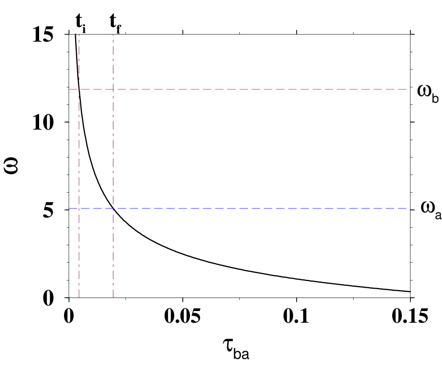
The problem of obtaining a closed form solution for the propagator ${\cal U}_{a}(t)$ has been transformed in to finding the solution of three coupled differential equations Eq. (116 ) which depend on $\omega(t)$ . A general solution has not been found but by choosing a particular functional form for $\omega(t)$ a closed form solution has been obtained.

III.3.3 The Explicit Solution for $\alpha$

To facilitate the solution of Eq. (116), a particular form of $\omega(t)$ is chosen:

\displaystyle\omega(t)=\frac{\dot{\alpha}_{1}}{\sqrt{2}}-J\frac{\sin(\alpha_{1})\sin(\alpha_{2})}{\cos(\alpha_{2})}~~~.

(121)

Two auxiliary functions are defined, $u(t)$ and $v(t)$ :

\displaystyle u(t)=-J^{2}t^{2}+\sqrt{2}rJt;~~v(t)=r-\sqrt{2}Jt~~~~.

(122)

$r$ is a constant which restricts the product $Jt$ : $\{~~0<r<1;~Jt<\sqrt{2}r\}$ . In terms of $u(t)$ and $v(t)$ , the solutions of Eq. (116) become:

\displaystyle\alpha_{1}~~=~~\arccos{\left(\frac{1}{\sqrt{1+2u}}\right)}~~~.

(123)

\displaystyle\alpha_{2}~~=~~\arcsin{\left(\frac{1}{1+r^{2}}(r\sqrt{1+2u}-v)\right)}~~~.

(124)

\displaystyle\alpha_{3}~~=~~-\frac{r}{2}\ln(2\sqrt{4u^{2}+2u}+4u+1)

\displaystyle-\frac{\sqrt{1-r^{2}}}{2}\{\arcsin\left(\frac{2r^{2}(1-r^{2})}{2u+1-r^{2}}+1-2r^{2}\right)-\frac{\pi}{2}\}-\{\arcsin{\left(\frac{v}{r}\right)}-\frac{\pi}{2}\}

\displaystyle-\frac{\sqrt{1-r^{2}}}{2}\{\arcsin{\left(\frac{1}{r}[1-\frac{1-r^{2}}{1+v}]\right)}+\arcsin{\left(\frac{1}{r}[1-\frac{1-r^{2}}{1-v}]\right)}\}~~~.

(125)

For $t=0$ , ${\bf\hat{U}}={\bf\hat{I}}$ , therefore $\alpha_{1}(0)=0,~\alpha_{2}(0)=0,~\alpha_{3}(0)=0$ which is consistent with Eq. (123),(124) and (125).

Introducing into Eqs. (121) the explicit functional forms of $\alpha_{k}$ , $\omega(t)$ becomes:

\displaystyle\omega(t)=\frac{Jv}{\sqrt{2}(1+2u)\sqrt{u}}-J\frac{\sqrt{2}\sqrt{u}(r\sqrt{1+2u}-v)}{\sqrt{1+2u}(\sqrt{1+2u}+rv)}~~~.

(126)

At $t=0$ , $\omega$ is singular. Since the engine operates between two finite values of $\omega$ a corresponding time segment is chosen which does not include the singularity at $t=0$ (Cf. Fig. 1). Using the group property of ${\cal U}_{a}(t)$ , i.e. ${\cal U}_{a}(t_{1}){\cal U}_{a}(t_{2})={\cal U}_{a}(t_{1}+t_{2})$ the propagation is carried out by changing the origin of time, ${\cal U}_{a}(t)~=~{\cal U}^{-1}_{a}(t_{0}){\cal U}_{a}(t+t_{0})$ where $t_{0}$ is either $t_{i}$ for the compression adiabat or $t_{f}$ for the expansion adiabat. One should note, that ${\cal U}^{-1}_{a}(t)={\cal U}^{\dagger}_{a}(t)$ but due to the explicit time dependence ${\cal U}^{-1}_{a}(t)\neq{\cal U}^{\dagger}_{a}(-t)$ .

Refer to caption — Figure 1: The external field $\omega$ as a function of time on the adiabats corresponding to the function Eq. (126) for which an analytic solution exist. Indicated are the values of the initial and the final time and of the corresponding $\omega$ which are used to construct the cycle of operation. Notice the singularity at $t=0$ .

IV Reconstruction of ${{{\boldsymbol{\mathrm{\rho}}}}}_{R}$

The reconstruction ${{{\boldsymbol{\mathrm{\rho}}}}}$ is designed to describe the state of the working medium from its initial state to equilibrium. As was analyzed in the previous section, the set of operators ${\bf\hat{B}}_{1},{\bf\hat{B}}_{2},{\bf\hat{B}}_{3},{\bf\hat{I}}$ are sufficient to describe the energy changes during the cycle of operation of the engine. Is this set sufficient to reconstruct the density operator?

In equilibrium ${{{\boldsymbol{\mathrm{\rho}}}}}^{eq}$ is diagonal in the energy representation, From the eigenvalues of the Hamiltonian Eq. (52), ${{{\boldsymbol{\mathrm{\rho}}}}}^{eq}$ in the energy picture becomes:

\displaystyle\begin{array}[]{c}\hat{\rho}^{eq}~~=\end{array}\left(\begin{array}[]{cccc}\frac{e^{\Omega\beta/\sqrt{2}}}{Z}&0&0&0\\ 0&\frac{1}{Z}&0&0\\ 0&0&\frac{1}{Z}&0\\ 0&0&0&\frac{e^{-\Omega\beta/\sqrt{2}}}{Z}\\ \end{array}\right)~~~,

where

\displaystyle Z~~=~~\exp{-(\Omega\beta/\sqrt{2})}~+~2~+~\exp{(\Omega\beta/\sqrt{2})}~=~\frac{{k\uparrow}}{{k\downarrow}}~+2+\frac{{k\downarrow}}{{k\uparrow}}~=~\frac{\Gamma^{2}}{{k\downarrow}{k\uparrow}}~~~.

(133)

By inspection, the diagonal elements of the equilibrium density operator are seen to be defined by three independent variables. The energy expectation accounts for one variable. The expectation value of ${\boldsymbol{\mathrm{\hat{B}}}}_{3}$ has no diagonal elements in the energy representation therefore two additional operators are required to facilitate a reproduction of ${\boldsymbol{\mathrm{\hat{\rho}}}}_{R}$ .

\displaystyle\begin{array}[]{c}{\bf\hat{B}}_{4}\end{array}~~=~~\begin{array}[]{c}2^{-3/2}\left({\boldsymbol{\mathrm{\hat{\sigma}}}}_{z}^{1}\otimes{\bf\hat{I}^{2}}-{\bf\hat{I}^{1}}\otimes{\boldsymbol{\mathrm{\hat{\sigma}}}}_{z}^{2}\right)\end{array}~~=~~~\frac{1}{\sqrt{2}}\left(\begin{array}[]{cccc}0&0&0&0\\ 0&1&0&0\\ 0&0&-1&0\\ 0&0&0&0\\ \end{array}\right)~~~,

and

\displaystyle{\bf\hat{B}}_{5}~=~\frac{1}{2}{\boldsymbol{\mathrm{\hat{\sigma}}}}_{z}^{1}\otimes{\boldsymbol{\mathrm{\hat{\sigma}}}}_{z}^{2}~=~\frac{1}{2}\left(\begin{array}[]{cccc}1&0&0&0\\ 0&-1&0&0\\ 0&0&-1&0\\ 0&0&0&1\\ \end{array}\right)~~~.

Since both ${\boldsymbol{\mathrm{\hat{B}}}}_{4}$ and ${\boldsymbol{\mathrm{\hat{B}}}}_{5}$ commute with the Hamiltonian, they undergo only dissipative dynamics but they are uninfluenced by the dephasing generated by $~{\cal L}_{D}^{*}$ :

\dot{\bf\hat{B}_{4}}~~=~~-\Gamma{\bf\hat{B}_{4}}

(146)

with the solution:

{\bf\hat{B}_{4}}(t)~~=~~{\bf\hat{B}_{4}}(0)\exp{(-\Gamma t)}~~~,

(147)

and $\langle{\bf\hat{B}_{4}^{eq}}\rangle=0$ . The equation of motion of $\bf\hat{B}_{5}$ is:

\dot{\bf\hat{B}_{5}}~~=~~-2\Gamma{\bf\hat{B}_{5}}-\sqrt{2}\frac{\omega}{\Omega}({k\downarrow}~-~{k\uparrow}){\bf\hat{B}_{1}}-\sqrt{2}\frac{\rm J}{\Omega}({k\downarrow}~-~{k\uparrow}){\bf\hat{B}_{2}}~~~=~~~

-2\Gamma{\bf\hat{B}_{5}}+~~2\Gamma\langle{\bf\hat{B}_{1}^{eq}}\rangle\bf\hat{B}_{1}~~+~~~2\Gamma\langle{\bf\hat{B}_{2}^{eq}}\rangle\bf\hat{B}_{2}~~~.

(148)

At equilibrium, $\dot{\bf\hat{B}_{5}}=0$ , and then $\langle{\bf\hat{B}_{5}^{eq}}\rangle~~=~~({\bf\hat{B}_{1}^{eq}})^{2}~~+~~({\bf\hat{B}_{2}^{eq}})^{2}$ , a result which can be verified by computing $\langle{\bf\hat{B}_{5}^{eq}}\rangle~~=~~~{\rm tr}\{{{\boldsymbol{\mathrm{\hat{\rho}}}}^{eq}}{\bf\hat{B}_{5}}\}$ . Eq. (148) is a linear first order inhomogeneous equation for ${\bf\hat{B}_{5}}$ depending on the time dependence of the closed set ${\bf\hat{B}_{1}},{\bf\hat{B}_{2}},{\bf\hat{B}_{3}}$ , Eq. (91). Changing Eq. (148) to observables, Eq. (1), and by integrating subject to the solutions of $b_{1}$ and $b_{2}$ leads to:

{b_{5}}(t)~=~\frac{2}{\Omega^{2}}\left(\omega(b_{1}(0)-b_{1}^{eq})+J(b_{2}(0)-b_{2}^{eq})\right)\left(\omega b_{1}^{eq}+J~b_{2}^{eq}\right)(e^{-\Gamma t}-e^{-2\Gamma t})~+~

k_{0}\left(k_{1}~c(e^{-(\Gamma+2\gamma\Omega^{2})t})~+~k_{2}~se^{-(\Gamma+2\gamma\Omega^{2})t}~-~k_{1}e^{-2\Gamma t}\right)~+~(b_{5}(0)-b_{5}^{eq})e^{-2\Gamma t}+b_{5}^{eq}~~~,

(149)

where:

k_{0}~~=~~\frac{2\Gamma(Jb_{1}^{eq}-\omega b_{2}^{eq})}{\Omega^{2}((\Gamma+2\gamma\Omega^{2})^{2}+2\Omega^{2})}

(150)

k_{1}~=~\left(J(b_{1}(0)-b_{1}^{eq})-\omega(b_{2}(0)-b_{2}^{eq})\right)(\Gamma+2\gamma\Omega^{2})-\Omega(b_{3}(0)-b_{3}^{eq})(\sqrt{2}\Omega)

and

k_{2}~=~\left(J(b_{1}(0)-b_{1}^{eq})-\omega(b_{2}(0)-b_{2}^{eq})\right)(\sqrt{2}\Omega)~+~\Omega(b_{3}(0)-b_{3}^{eq})(\Gamma+2\gamma\Omega^{2})~~~.

Using the set of of the five orthogonal and normalized operators together with the identity operator the density operator ${\boldsymbol{\mathrm{\hat{\rho}}}}_{R}$ is reconstructed. Representing ${\boldsymbol{\mathrm{\hat{\rho}}}}_{R}$ in different basses facilitates the calculation of the different entropies. ${\boldsymbol{\mathrm{\hat{\rho}}}}_{R}$ in the polarization basis becomes:

\displaystyle\begin{array}[]{c}{{\boldsymbol{\mathrm{\hat{\rho}}}}_{p}}\end{array}~~=~~~\left(\begin{array}[]{cccc}\frac{1}{4}+\frac{{b_{1}}}{\sqrt{2}}+\frac{b_{5}}{2}&0&0&\frac{{b_{2}}}{\sqrt{2}}-i\frac{{b_{3}}}{\sqrt{2}}\\ 0&\frac{1}{4}+\frac{b_{4}}{\sqrt{2}}-\frac{b_{5}}{2}&0&0\\ 0&0&\frac{1}{4}-\frac{b_{4}}{\sqrt{2}}-\frac{b_{5}}{2}&0\\ \frac{{b_{2}}}{\sqrt{2}}+i\frac{{b_{3}}}{\sqrt{2}}&0&0&\frac{1}{4}-\frac{b_{1}}{\sqrt{2}}+\frac{b_{5}}{2}\\ \end{array}\right)~~~.

The off diagonal elements of ${{\boldsymbol{\mathrm{\hat{\rho}}}}_{p}}$ are the expectation values of the operators:
${{\boldsymbol{\mathrm{\hat{B}}}}}_{\pm}=\frac{1}{\sqrt{2}}({\boldsymbol{\mathrm{\hat{B}}}}_{2}\pm i{\boldsymbol{\mathrm{\hat{B}}}}_{3})$ which represent the correlation between the individual spins.

The density operator ${\boldsymbol{\mathrm{\hat{\rho}}}}_{R}$ in the energy basis becomes:

\displaystyle\begin{array}[]{c}{\boldsymbol{\mathrm{\hat{\rho}}}}_{e}\end{array}~~=~~~\left(\begin{array}[]{cccc}\frac{1}{4}-\frac{E}{\Omega\sqrt{2}}+\frac{b_{5}}{2}&0&0&+\frac{ib_{3}}{\sqrt{2}}-\frac{Jb_{1}}{\Omega\sqrt{2}}+\frac{\omega b_{2}}{\Omega\sqrt{2}}\\ 0&\frac{1}{4}+\frac{b_{4}}{\sqrt{2}}-\frac{b_{5}}{2}&0&0\\ 0&0&\frac{1}{4}-\frac{b_{4}}{\sqrt{2}}-\frac{b_{5}}{2}&0\\ -\frac{ib_{3}}{\sqrt{2}}-\frac{Jb_{1}}{\Omega\sqrt{2}}+\frac{\omega b_{2}}{\Omega\sqrt{2}}&0&0&\frac{1}{4}+\frac{E}{\Omega\sqrt{2}}+\frac{b_{5}}{2}\\ \end{array}\right)~~~,

where $E=\omega b_{1}+Jb_{2}$ . In equilibrium, the off-diagonal elements vanish, and the matrix will be identical to Eq. (IV). In non-equilibrium, the off-diagonal elements of ${{{\boldsymbol{\mathrm{\rho}}}}}_{e}$ determine the ”phase” Cf. Sec. VIII.

To compute the Von-Neumann entropy ${{{\boldsymbol{\mathrm{\rho}}}}}_{R}$ is diagonalized leading to:

\displaystyle\begin{array}[]{c}\hat{\rho}_{vn}\end{array}~~=~~~\left(\begin{array}[]{cccc}\frac{1}{4}-\frac{D}{\sqrt{2}}+\frac{b_{5}}{2}&0&0&0\\ 0&\frac{1}{4}+\frac{b_{4}}{\sqrt{2}}-\frac{b_{5}}{2}&0&0\\ 0&0&\frac{1}{4}-\frac{b_{4}}{\sqrt{2}}-\frac{b_{5}}{2}&0\\ 0&0&0&\frac{1}{4}+\frac{D}{\sqrt{2}}+\frac{b_{5}}{2}\\ \end{array}\right)~~~,

where $D=\sqrt{b_{1}^{2}+b_{2}^{2}+b_{3}^{2}}$ .

V Dynamical Temperature ( $T_{dyn}$ ) on the branches

Based on the definition of the dynamical temperature $T_{dyn}$ in Eq. (21), and from Eq. (III.1.2):

\displaystyle T_{dyn}~=~\frac{\dot{\omega}b_{1}+\omega\dot{b}_{1}+J\dot{b}_{2}}{-\sum\dot{p}_{i}^{E}(1+\log(p_{i}^{E}))}~=~\frac{\dot{\omega}b_{1}-\Gamma E-\frac{\Omega}{\sqrt{2}}(k\downarrow-k\uparrow)}{-\sum\dot{p}_{i}^{E}(1+\log(p_{i}^{E}))}~~~,

(169)

The four probabilities $p_{i}^{E}$ are the diagonal elements of the density operator in the energy representation ${{{\boldsymbol{\mathrm{\rho}}}}}_{e}$ , Eq. (IV). The derivatives of the probabilities are obtained from Eqs. (III.1.3) and (148):

\displaystyle\dot{p}_{1}^{E}=\frac{-\dot{\omega}b_{1}+\Gamma E}{\Omega\sqrt{2}}+\frac{(k\downarrow-k\uparrow)}{2}+\frac{\dot{b}_{5}}{2},~~\dot{p}_{2}^{E}=-\frac{\dot{b}_{5}}{2},~~

\displaystyle\dot{p}_{3}^{E}=-\frac{\dot{b}_{5}}{2},~~\dot{p}_{4}^{E}=\frac{\dot{\omega}b_{1}-\Gamma E}{\Omega\sqrt{2}}-\frac{(k\downarrow-k\uparrow)}{2}+\frac{\dot{b}_{5}}{2}~~~,

(170)

where ${\dot{b}_{5}}$ is obtained form Eq. (148): $\dot{b}_{5}~=~2\Gamma(b_{1}^{eq}b_{1}+b_{2}^{eq}b_{2}-b_{5})$ .

V.1 Dynamical temperature on the $\it isochores$

Evaluating the derivatives of the probabilities in Eqs. (170) and using the fact that on the isochores $\dot{\omega}$ =0, the dynamical temperature, Eq. (169), becomes:

\displaystyle T_{dyn}~=~\frac{\left(\Gamma E+\frac{\Omega}{\sqrt{2}}(k\downarrow-k\uparrow)\right)}{\left(\frac{\Gamma E}{\Omega\sqrt{2}}\log(p_{1}/p_{4})+\frac{(k\downarrow-k\uparrow)}{2}\log(p_{1}/p_{4})+\frac{1}{2}\dot{b}_{5}\log(p_{1}p_{4}/p_{2}p_{3})\right)}~~~.

(171)

A consistency check is obtained by comparing $T_{dyn}$ for J=0 with the internal temperature of a two-level-system. For $J=0$ :

\displaystyle T_{dyn}~=\frac{\omega}{\sqrt{2}\log(\frac{1/2+b_{1}/\sqrt{2}}{1/2-b_{1}/\sqrt{2}})}~~~,

(172)

which leads to:

\displaystyle b_{1}~=~-1/\sqrt{2}\frac{k\downarrow-k\uparrow}{k\downarrow+k\uparrow}~=~-1/\sqrt{2}\tanh(\frac{\omega}{\sqrt{2}T_{dyn}})~~~.

(173)

which is the internal temperature for a noninteracting spin system with energy spacing $\omega/\sqrt{2}$ geva0.

V.2 Dynamical temperature on the $\it adiabats$

On the adiabats $\dot{b}_{4}=$ and $\dot{b}_{5}=0$ . From Eq. (169) and (170) the derivatives of the probabilities on the adiabats become:

\displaystyle\dot{p}_{1}^{E}~=~-~\frac{\dot{\omega}}{\Omega\sqrt{2}};~~\dot{p}_{2}^{E}~=~0;~~\dot{p}_{3}^{E}~=~0;~~\dot{p}_{4}^{E}~=~\frac{\dot{\omega}}{\Omega\sqrt{2}}~~~,

(174)

which leads to the dynamical temperature on the ${\it adiabats}$ :

\displaystyle T_{dyn}^{ad}~=\frac{\Omega\sqrt{2}}{\log(\frac{p_{1}^{E}}{p_{4}^{E}})}~~~.

(175)

VI The Thermodynamic quantities for the coupled spin fluid

•

The heat absorbed or delivered by the heat engine

Using Eq.(15) the heat ${\cal Q}\rm_{h/c}$ absorbed or delivered becomes:

$\displaystyle{\cal Q}\rm_{i}~=~\rm(\exp({-\Gamma\tau_{i}})-1)(\omega_{i}b_{1}+Jb_{2})$ (176)

where $i=h/c$
•

The work absorbed or delivered by the heat engine

The power, Eq. (14), is $\langle\frac{\partial H}{\partial t}\rangle=B_{1}(t)\dot{\omega}$ . Therefore, the work becomes:

$\displaystyle\cal W~=~\rm\int_{\tau i}^{\tau f}b_{1}\dot{\omega}dt~~~.$ (177)
•

Entropy production.

The entropy production per cycle, ${\cal DS}_{cycle}$ , created on the boundaries becomes (Cf. Eq. (17)):

$\displaystyle{\cal DS}_{cycle}=-\left({\cal Q}\rm_{AB}/T_{h}+{\cal Q}\rm_{CD}/T_{c}\right)~~~.$ (178)

•

$\bf Efficiency.$

The efficiency per cycle, $\eta_{cycle}$ is:

\displaystyle\eta_{cycle}=\cal W~/{\cal Q}\rm_{AB}=\frac{\int_{\tau i}^{\tau f}b_{1}\dot{\omega}dt}{\rm(\exp({-\Gamma\tau_{i}})-1)(\omega_{i}b_{1}+Jb_{2})}~~~.

(179)

The maximal efficiency of the engine is:

1-\frac{\Omega_{a}}{\Omega_{b}}~=~1-\frac{\sqrt{\omega^{2}_{a}+J^{2}}}{\sqrt{\omega^{2}_{b}+J^{2}}}~~~.

The upper bound should be the Carnot’s efficiency, a bound correct for all J and the fact that $\frac{\omega_{a}}{\omega_{b}}~>~\frac{T_{c}}{T_{h}}$ :

\displaystyle 1-\frac{\omega^{2}_{a}+J^{2}}{\omega^{2}_{b}+J^{2}}~<~1-\frac{\omega^{2}_{a}}{\omega^{2}_{b}}~<~1-\frac{T^{2}_{c}}{T^{2}_{h}}~~~.

(180)

VII The Cycle of Operation: The Otto cycle

The operation of the heat engine is determined by the properties of the working medium and by the hot and cold baths. These properties are summarized by the generator of the dynamics ${\cal L}$ . The cycle of operation is defined by the external controls which include the variation in time of the field with the periodic property $\omega(t)=\omega(t+\tau)$ where $\tau$ is the total cycle time synchronized with the contact times of the working medium with the hot and cold baths $\tau_{h}$ and $\tau_{c}$ . In this study a specific operating cycle composed of two branches termed isochores where the field is kept constant and the working medium is in contact with the hot/cold baths. In addition two branches termed adiabats where the field $\omega(t)$ varies and the working medium is disconnected from the baths. This cycle is a quantum analogue of the Otto cycle.

The dynamics of the working medium has been described in Sec. III. The parameters defining the cycle are:

•

$T_{h}$ and $T_{b}$ , the hot/cold bath temperatures.
•

$\Gamma_{h}$ and $\Gamma_{c}$ , the hot/cold bath heat conductance parameters.
•

$\gamma_{h}$ and $\gamma_{c}$ , the hot/cold bath dephasing parameters.
•

$J$ -the strength of the internal coupling

The external control parameter define the four strokes of the cycle (Cf. Fig. 2):

1.

Isochore $A\rightarrow B$ : when the field is maintained constant, $\omega=\omega_{b}$ , the working medium is in contact with the hot bath for a period of $\tau_{h}$ .
2.

Adiabat $B\rightarrow C$ : when the field changes linearly from $\omega_{b}$ to $\omega_{a}$ in a time period of $\tau_{ba}$ .
3.

Isochore $C\rightarrow D$ : when the field is maintained constant $\omega=\omega_{a}$ the working medium is in contact with the cold bath for a period of $\tau_{c}$ .
4.

Adiabat $C\rightarrow A$ : when the field changes linearly from $\omega_{a}$ to $\omega_{b}$ in a time period of $\tau_{ab}$ .

The trajectory of the cycle in the field and the entropy plane ( $\omega,{\cal S}_{E}$ ) is shown in Fig. 2 employing a numerical propagation with a linear $\omega$ dependence on time.

A different perspective on the dynamics during the cycle of operation is shown in Fig. 3, displaying the cycle trajectory in the $b_{1},b_{2},b_{3}$ coordinates. The hypothetical cycle with infinitely long time on all branches would include the equilibrium points E and F. The cycle trajectory is planar on the ${\bf\hat{B}_{3}}=0$ plane as can be seen in panel C. The cycle ABCD with finite time allocation spirals around the infinitely long time cycle with an incursion into the ${\bf\hat{B}_{3}}$ directions.

The reference cycle with infinite time allocation on all branches is characterized by a diagonal state ${{{\boldsymbol{\mathrm{\rho}}}}}_{e}$ in the instantaneous energy representation. The slow motion on the adiabats allows the state ${{{\boldsymbol{\mathrm{\rho}}}}}$ to adopt to the changes in time of the Hamiltonian, which therefore can be termed adiabatic following. If the time allocation on the adiabats is short, non-adiabatic effects take place. In the sudden limit of infinite short time allocation on the adiabat, the state of the system has no time to evolve ${{{\boldsymbol{\mathrm{\rho}}}}}(t_{i}+\tau_{ab})={{{\boldsymbol{\mathrm{\rho}}}}}(t_{i})$ . The Hamiltonian will then change from ${\bf\hat{H}_{i}}=\omega(t_{i}){\bf\hat{B}_{1}}+J{\bf\hat{B}_{2}}$ to ${\bf\hat{H}_{f}}=\omega(t_{i}+\tau_{ab}){\bf\hat{B}_{1}}+J{\bf\hat{B}_{2}}$ therefore the representation of the state ${{{\boldsymbol{\mathrm{\rho}}}}}_{e}(t_{i}+\tau_{ab})$ in the new energy representation is rotated by an angle $\theta=(\theta_{i}-\theta_{f})$ compared to the former one. Where, $\theta_{i}=\arcsin(J/\Omega(t_{i}))$ and $\theta_{f}=\arcsin\left(J/\Omega(t_{i}+\tau_{ab})\right)$ .

When following the direction of the cycle, the energy-entropy increases on the adiabts. This is evident in both Fig. 2 and Fig. 4. This entropy increase is the signature of nonadiabatic effects reflecting the inability of the population on the energy states to follow the change in time of the Hamiltonain. As a result the energy dispersion increases. Since the evolution on these branches is unitary, ${\cal S}_{VN}$ is constant. When more time is allocated to the adiabats the increase in ${\cal S}_{E}$ is smaller. For infinite time allocation ${\cal S}_{E}~~=~~{\cal S}_{VN}$ . In this case the state of the woking medium is always diagonal in the energy representation. The larger curvature of the entropy increase in the analytic result of Fig. 4, compared with the numerical result of Fig. 2 reflects the difference in the dependence of $\omega(t)$ on time. When the analytic functional form of $\omega(t)$ is used in the numerical propagation the numerical solution converges to the values of the analytic solution. This convergence test was used as a consistancy check for both methods. Convergence was not uniform for all elements in the propagator (Cf. Eq. (III.3.1) and Eq. (III.3.2) ). Comparing the elements of the numerical propagator ${\cal U}_{a}(\tau_{ab})$ to the elements of analytic ${\cal U}_{a}(\tau_{ab})$ , showed that the largest discrepency between the individual elements at $t=\tau_{ab}$ was less than $10^{-3}$ when a time step of $\Delta t=\tau_{ab}/1000$ was used.

In Fig. 5 the cycle of operation is presented in the energy-entropy internal-temperature coordinates $({\cal S}_{E},T_{dyn})$ . The cycles shown corresponds to the analyticial cycles of Fig. 4. The discontinuities in the short time cycle reflect over-heating in the compression stage as shown as the difference between the point A and A’ in Fig. 5. The heat accumulated is quenched when the working medium is put in contact with the hot bath. This phenomena has been identified in measurements of working fluid temperatures in actual heat engines or heat pumps gordon98. A discontinuity as a result of insufficient cooling of the woking medium in the expansion branch is also evident in the short time cycle. The magnitude of these discontinuities is reduced at longer times and dissapear for the infinite long cycle where the working fluid reaches thermal equilibrium with the hot bath at point $\bf E$ and with the cold bath at point $\bf F$ . In this case both adiabatic branches are isoentropic.

It is clear from Fig. 5, that for the cycles with vertical adiabats the work is the area enclosed by the cycle trajectory. When the time allocation on the adiabats is restricted this is no longer the case since due to the entropy increase, the area under the hot isochore does not cover the area under the cold isochore. Additional cooling is then required to dissipate the extra work required to drive the system on the adiabats at finite time.

VIII The effect of phase and dephasing.

The performence of the heat engine explicitly depend on heat and work which constitute the energy (16). Do other observables, incompatiable with the energy, influence the engins performence? Examining the cycle trajectory on the isochores in Fig. 3, in addition to the motion in the energy direction, towoard equilibration, spiraling motion exists. This motion is characterized by amplitude and phase of an observable in the plane perpendicular to the energy direction. The phase $\phi$ of this motion advances in time, i.e. $\phi\propto t$ . The concept of phase has its origins in classical mechanics where a canonincal trnsformation leads to a new set of action angle variables. The conjugate variable to the Hamiltonain is the phase. In quantum mechanics the phase observable has been a subject of contineous debate nieto68. For a harmonic oscillator it is related to the creation and anhilation operator $\bf\hat{a}$ levyleblond; gour02. In analogy the raising/lowering operator is defined:

{\bf\hat{L}}_{\pm}~~=~~\frac{1}{\sqrt{2}\Omega}\left(-J{\bf\hat{B}_{1}}+\omega{\bf\hat{B}_{2}}\pm i\Omega{\bf\hat{B}_{3}}\right)~~~,

(181)

which has the following commutation relation with the Hamiltonian:

[{\bf\hat{H}},{\bf\hat{L}}_{\pm}]=\pm\sqrt{2}\Omega{\bf\hat{L}}_{\pm}~~~.

(182)

The free evolution of $\bf\hat{L}_{+}$ therefore becomes: $\bf\hat{L}_{+}(t)=e^{i\sqrt{2}\Omega t}{\bf\hat{L}}_{+}(0)$ which defines the phase variable through: $\langle{\bf\hat{L}_{+}}\rangle~=~re^{i\phi}$ , therefore $\phi=\arctan\left(\frac{\Omega b_{3}}{-Jb_{1}+\omega b_{2}}\right)$ . A corroboration for this interpretation is found by examining the state ${{{\boldsymbol{\mathrm{\rho}}}}}_{e}$ in the energy representation (Cf. Eq. (IV). The off diagonal elements are completely specified by the expectation values of ${\bf\hat{L}}_{\pm}$ .

The dynamics of ${\bf\hat{L}}_{\pm}$ on the isochores includes also dissipative contributions which can be evaluated using Eq. (III.1.3):

\dot{\bf\hat{L}}_{\pm}~~=~~\pm i\sqrt{2}\Omega{\bf\hat{L}}_{\pm}-\left(\Gamma+2\gamma\Omega^{2}\right){\bf\hat{L}}_{\pm}

(183)

Examining Eq. (183) it is clear that the amplitude of ${\bf\hat{L}}_{\pm}$ decays exponentially with the rate $\frac{1}{T_{2}}=\Gamma+2\gamma\Omega^{2}$ , where $\Gamma$ is the dephasing contribution due to energy relaxation and $\frac{1}{T_{2}^{*}}=2\gamma\Omega^{2}$ is the pure dephasing contribution.

Both Fig. 3 and Fig. 6 show that the dephasing is not complete at the end of the isochores. A small change in the time allocation in the order of $1/\Omega$ can completely change the final phase on the isochore and on the initial phase for the adiabat. This means that the cycle performance characteristic becomes very sensitive to small changes in time allocation on the isochores. This effect can be observed in Fig. 7 for the power and Fig. 8 for the entropy production.

Examining Fig. 7 reveals that increasing $J$ increases the ”phase” effect. For $J=2$ for specific time allocations the power can even become negative. Increasing the dephasing rate either by adding pure dephasing or by changing the heat transfer rate reduces the ”noise”. This can also be seen in Fig. 8.

An interesting phase effect can be observed in Fig. 9 where the cycle is displayed in the $({\cal S}_{E},T_{dyn})$ plane. The inner (solid black) cycle shows an energy-entropy decrease in the compression adiabat. The reason for this decrease is a phase memory from the compression adiabat which is due to insufficient dephasing on the cold isochore. Additional pure dephasing eliminates this entropy decrease as can be seen in the dashed black cycle. This cycle is also pushed to larger entropy values. The orange cycles are characterized by a longer time allocation on the isochores. For these cycles the energy-entropy always increases on the adiabats. This cycle is shifted by dephasing to lower energy-entropy values.

IX discussion

Quantum thermodynamics is the study of thermodynamical phenomena based on quantum mechanical principles hoffmann. To meet this challenge, quantum expectation values have to be related to thermodynamical variables. The Otto cycle is an ab-initio quantum model for which analytic solutions have been obtained. The principle thermodynamical variables: energy entropy and temperature are derived from first principles. The solution of the quantum equations of motion for the state ${{{\boldsymbol{\mathrm{\rho}}}}}$ , enables tracing the thermodynamical variables for each point on the cycle trajectory. This dynamical picture supplies a rigorous formalism for finite-time-thermodynamics salamon77; andresen83.

An underlying principle of finite-time-thermodynamics is that operation irreversibilities are inevitable if a process is run at finite rate. Moreover these irreversibilities are the source of performance limitations imposed on the process. The present Otto cycle heat engine in line with FTT is subject to two major performance limitations:

•

Finite rate of heat transfer from the hot bath to the working medium and from the working medium to the cold bath.
•

Additional work invested in the expansion and compression branches is required to drive the adiabats at a finite time.

The finite rate of heat transfer limits the maximum obtainable power ${\cal P}$ curzon75. The present Otto engine model is not an exception, showing similarities with previous studies of discrete quantum heat engines feldmann96; feldmann00; geva0; geva1.

The irreversibility caused by the finite time duration on the adiabats is the novel finding of the present study as well as the preceding short letter kosloff01. This irreversibility is closely linked to the quantum adiabatic condition. The nonadiabatic irreversibility is caused by the interplay of the noncommutability of the Hamiltonian at different points along the cycle trajectory and the dephasing caused by coupling to the heat baths on the isochores. In the present Otto cycle these contributions are separated in time. The non-adiabaticity can be characterized by an increase in the modulus of $\langle{\bf\hat{L}}_{\pm}\rangle$ on the adiabats. Dephasing, i.e. exponential decay of the modulus of $\langle{\bf\hat{L}}_{\pm}\rangle$ is induced by the coupling to the baths on the isochores.

The dynamics of the ${\bf\hat{L}}_{\pm}$ operator associated with the phase can be compared to the ${\bf\hat{B}}_{\pm}$ operator associated with the internal correlation between the spins (Cf. (IV)). The absolute value of $|\bf\hat{B}_{\pm}|$ oscillates on all branches of the cycle never reaching zero. This is not surprising since $\bf\hat{B}_{\pm}$ does not commute with the Hamiltonian. The ”angle” $\phi_{B}=\arctan({b_{3}/b_{2}})$ is excited for small cycle times. For cycles with large time allocation on the isochores, $\phi_{B}$ is found to be close to zero. These observations reflect the two types of correlations between particles. A ”classical” correlation and a quantum correlation meaning EPR EPR; lindblad73 entanglement between particles. The general trend is therefore for the engine to become more ”classical” when the cycle times become longer. In this case the state follows the energy direction and in addition entanglement between particles is small. Adding pure dephasing has a similar effect. A continuous measurement of energy during operation will also lead to effective pure dephasing. For short cycle times quantum effects become important. The entropy decrease on the adiabats which is the result of ”phase” memory is such an example. The quantum effect which influences the performance is the excess work on the adiabat due to the inability of the state to follow the energy direction.

Acknowledgements.

This research was supported by the US Navy under contract number N00014-91-J-1498 and the Israel Science Foundation. The authors wish to thank Lajos Diosi and Jeff Gordon for their continuous support and help.

Appendix A The F operators

The method of construction of $\bf\hat{F}_{\rm j}$ is based on identifying the operators with the raising and lowering operators in the energy frame. The matrix ${\cal C}$ which diagonalizes the Hamiltonian becomes:

\displaystyle\begin{array}[]{c}{\cal C}\end{array}~~=~\left(\begin{array}[]{cccc}-\sqrt{\frac{\Omega-\omega}{2\Omega}}&0&0&\sqrt{\frac{\Omega+\omega}{2\Omega}}\\ 0&1&0&0\\ 0&0&1&0\\ \sqrt{\frac{\Omega+\omega}{2\Omega}}&0&0&\sqrt{\frac{\Omega-\omega}{2\Omega}}\\ \end{array}\right)

Denoting $\sqrt{\frac{\Omega-\omega}{2\Omega}}~=~\mu~~$ , and $\sqrt{\frac{\Omega+\omega}{2\Omega}}~=~\chi~~~$ , the diagonalization of the Hamiltonian matrix becomes:

\displaystyle\left(\begin{array}[]{cccc}-\mu&0&0&\chi\\ 0&1&0&0\\ 0&0&1&0\\ \chi&0&0&\mu\\ \end{array}\right)\left(\begin{array}[]{cccc}\frac{\omega}{\sqrt{2}}&0&0&\frac{J}{\sqrt{2}}\\ 0&0&0&0\\ 0&0&0&0\\ \frac{J}{\sqrt{2}}&0&0&-\frac{\omega}{\sqrt{2}}\\ \end{array}\right)\left(\begin{array}[]{cccc}-\mu&0&0&\chi\\ 0&1&0&0\\ 0&0&1&0\\ \chi&0&0&\mu\\ \end{array}\right)~~=~~\left(\begin{array}[]{cccc}-\frac{\Omega}{\sqrt{2}}&0&0&0\\ 0&0&0&0\\ 0&0&0&0\\ 0&0&0&\frac{\Omega}{\sqrt{2}}\\ \end{array}\right)

The down transition rates $k\downarrow$ are chosen to be equal for all the four transitions, while the raising transitions $k\uparrow$ comply with detailed balance. Schematically the eight transitions are:

\displaystyle\begin{array}[]{cccccccc}\bf F_{1}&\bf F_{2}&\bf F_{3}&\bf F_{4}&\bf F_{5}&\bf F_{6}&\bf F_{7}&\bf F_{8}\\ E_{2}&E_{2}&E_{3}&E_{3}&E_{4}&E_{4}&E_{4}&E_{4}\\ \Uparrow&\Downarrow&\Uparrow&\Downarrow&\Uparrow&\Downarrow&\Uparrow&\Downarrow\\ E_{1}&E_{1}&E_{1}&E_{1}&E_{2}&E_{2}&E_{3}&E_{3}\\ \end{array}

A.0.1 Detailed presentation of a few $F_{i}$ operators.

The $\bf\hat{F}$ operator for the transition $E_{1}$ to $E_{2}$ , is $\bf F_{1\rightarrow 2}\equiv\bf F_{1}$ ; In the energy picture, it is simply:

\displaystyle\begin{array}[]{c}\bf F_{1}~~=\end{array}\sqrt{k\downarrow}\left(\begin{array}[]{cccc}0&0&0&0\\ 1&0&0&0\\ 0&0&0&0\\ 0&0&0&0\\ \end{array}\right)

Using the matrix ${\cal C}$ to transform back to the polarization picture leads to:

\displaystyle\begin{array}[]{c}\bf F_{1}~~=\end{array}\sqrt{k\downarrow}\left(\begin{array}[]{cccc}-\mu&0&0&\chi\\ 0&1&0&0\\ 0&0&1&0\\ \chi&0&0&\mu\\ \end{array}\right)\left(\begin{array}[]{cccc}0&0&0&0\\ 1&0&0&0\\ 0&0&0&0\\ 0&0&0&0\\ \end{array}\right)\left(\begin{array}[]{cccc}-\mu&0&0&\chi\\ 0&1&0&0\\ 0&0&1&0\\ \chi&0&0&\mu\\ \end{array}\right)~~=~

\displaystyle\sqrt{k\downarrow}\left(\begin{array}[]{cccc}0&0&0&0\\ -\mu&0&0&\chi\\ 0&0&0&0\\ 0&0&0&0\\ \end{array}\right)

And $\bf F_{1}^{\dagger}$ will be;

\displaystyle\begin{array}[]{c}\bf F_{1}^{\dagger}~~=\end{array}\sqrt{k\downarrow}\left(\begin{array}[]{cccc}-\mu&0&0&\chi\\ 0&1&0&0\\ 0&0&1&0\\ \chi&0&0&\mu\\ \end{array}\right)\left(\begin{array}[]{cccc}0&1&0&0\\ 0&0&0&0\\ 0&0&0&0\\ 0&0&0&0\\ \end{array}\right)\left(\begin{array}[]{cccc}-\mu&0&0&\chi\\ 0&1&0&0\\ 0&0&1&0\\ \chi&0&0&\mu\\ \end{array}\right)~~=~~

\displaystyle\sqrt{k\downarrow}\left(\begin{array}[]{cccc}0&-\mu&0&0\\ 0&0&0&0\\ 0&0&0&0\\ 0&\chi&0&0\\ \end{array}\right)

Using a similar procedure all the $\bf\hat{F}_{i}$ in the polarization picture become:

\displaystyle\begin{array}[]{c}{\bf\hat{F}_{1}}~~=~~{\bf\hat{F}}_{1\rightarrow 2}~~=\end{array}\sqrt{k\downarrow}\left(\begin{array}[]{cccc}0&0&0&0\\ -\mu&0&0&\chi\\ 0&0&0&0\\ 0&0&0&0\\ \end{array}\right)

\displaystyle\begin{array}[]{c}{\bf\hat{F}_{2}}~~=~~{\bf\hat{F}}_{2\rightarrow 1}~~=\end{array}\sqrt{k\uparrow}\left(\begin{array}[]{cccc}0&-\mu&0&0\\ 0&0&0&0\\ 0&0&0&0\\ 0&\chi&0&0\\ \end{array}\right)

\displaystyle\begin{array}[]{c}{\bf\hat{F}}_{3}~~=~~\bf F_{1\rightarrow 3}~~=\end{array}\sqrt{k\downarrow}\left(\begin{array}[]{cccc}0&0&0&0\\ 0&0&0&0\\ -\mu&0&0&\chi\\ 0&0&0&0\\ \end{array}\right)

\displaystyle\begin{array}[]{c}{\bf\hat{F}_{4}}~~=~~{\bf\hat{F}}_{3\rightarrow 1}~~=\end{array}\sqrt{k\uparrow}\left(\begin{array}[]{cccc}0&0&-\mu&0\\ 0&0&0&0\\ 0&0&0&0\\ 0&0&\chi&0\\ \end{array}\right)

\displaystyle\begin{array}[]{c}{\boldsymbol{\mathrm{\hat{F}}}}_{5}~~=~~{\boldsymbol{\mathrm{\hat{F}}}}_{2\rightarrow 4}~~=\end{array}\sqrt{k\downarrow}\left(\begin{array}[]{cccc}0&\chi&0&0\\ 0&0&0&0\\ 0&0&0&0\\ 0&\mu&0&0\\ \end{array}\right)

\displaystyle\begin{array}[]{c}{\boldsymbol{\mathrm{\hat{F}}}}_{6}~~=~~{\boldsymbol{\mathrm{\hat{F}}}}_{4\rightarrow 2}~~=\end{array}\sqrt{k\uparrow}\left(\begin{array}[]{cccc}0&0&0&0\\ \chi&0&0&\mu\\ 0&0&0&0\\ 0&0&0&0\\ \end{array}\right)

\displaystyle\begin{array}[]{c}{\boldsymbol{\mathrm{\hat{F}}}}_{7}~~=~~{\boldsymbol{\mathrm{\hat{F}}}}_{3\rightarrow 4}~~=\end{array}\sqrt{k\downarrow}\left(\begin{array}[]{cccc}0&0&\chi&0\\ 0&0&0&0\\ 0&0&0&0\\ 0&0&\mu&0\\ \end{array}\right)

\displaystyle\begin{array}[]{c}{\boldsymbol{\mathrm{\hat{F}}}}_{8}~~=~~{\boldsymbol{\mathrm{\hat{F}}}}_{4\rightarrow 3}~~=\end{array}\sqrt{k\uparrow}\left(\begin{array}[]{cccc}0&0&0&0\\ 0&0&0&0\\ \chi&0&0&\mu\\ 0&0&0&0\\ \end{array}\right)

References

(1) S. Carnot, Réflections sur la Puissance Motrice du Feu et sur les Machines propres à Développer cette Puissance (Bachelier, Paris, 1824).
(2) L. Szilard, Z. Physik 53, 840 (1929).
(3) Leon Brillouin, ”Science and Information Theory”, Academic Press, 1956.
(4) R. Kosloff and T. Feldmann, Phys. Rev. E 65, 055102 (2002).
(5) T. Feldmann, E. Geva, R. Kosloff and P. Salamon, Am. J. Phys. 64, 485 (1996).
(6) T. Feldmann and R. Kosloff, Phys. Rev. E 61, 4774 (2000).
(7) S. Lloyd, Phys. Rev. A 56 3374 (1997).
(8) J. Geusic, E. S. du Bois, R. D. Grasse, and H. Scovil, J. Appl. Phys., 30, 1113 (1959).
(9) R. Kosloff, J. Chem. Phys., 80, 1625 (1984).
(10) E. Geva and R. Kosloff, J. Chem. Phys., 96, 3054 (1992).
(11) E. Geva and R. Kosloff, J. Chem. Phys., 97, 4398 (1992).
(12) E. Geva and R. Kosloff, J. Chem. Phys., 104, 7681 (1996).
(13) J. C. Chen, B. H. Lin and B. Hua, J. Phys. D Applied Physics 35, 2051 (2002).
(14) C. M. Bender, D. C. Brody and B. K. Meister, J. Phys. A 33 4427 (2000).
(15) C. M. Bender, D. C. Brody and B. K. Meister, Poc. Roy. Soc. of London Ser. A 458 1519 (2002).
(16) R. Kosloff, E. Geva and J. M. Gordon, J. Appl. Phys. 87, 8093 (2000).
(17) J. P. Palao, R. Kosloff and J. M. Gordon, Phys. Rev. E 64, 056130-8 (2001).
(18) E. Geva, J. Mod. Opt. 49, 635 (2002)
(19) F. L. Curzon and B. Ahlborn, Am. J. Phys. 43, 22 (1975).
(20) A. Ben-Shaul and R.D. Levine, J. Non-Equilib. Thermodyn. 4, 363 (1979).
(21) P. Salamon, J. D. Nulton, G. Siragusa, T. R. Andersen and A. Limon Energy, 26, 307 (2001).
(22) P. Salamon, A. Nitzan, B. Andresen and R. S. Berry Phys. Rev. A 21, 2115 (1980).
(23) J. M. Gordon and M. Huleihil, J. Appl. Phys. 69, 1 (1991).
(24) B. Andresen, ”Finite-Time Thermodynamics”, (Phys. Lab II. University of Copenhagen, Copenhagen 1983).
(25) A. Bejan, ”Entropy Generation Minimization”, (Chemical Rubber Corp., Boca Raton FL. 1996).
(26) K. C. Ng, H. T. Chua, K. Tu, J. M. Gordon, T. Kashiwagi, A Akisawa and B. B. Saha, J. Appl. Phys. 83, 1831 (1998).
(27) K. Lendi and A. J. van Wonderen, J. Phys. A Math. Gen. 34, 1285 (2001).
(28) G. Lindblad, Commun. Math. Phys., 48, 119 (1976).
(29) Y. Alhasid, R. D. Levine, Phys. Rev. A 18, 89 (1978).
(30) B. G. Adams, J. Cizek and J. Paldus, ”Lie Algebraic Methods and Their application to Simple Quantum Systems” Adv. Quantum. Chem. 19, 1 (1988).
(31) B. G. Wybourne, ”Classical Groups for Physics” Wiley (1973).
(32) R. Alicki and K. Lendi, Quantum Dynamical Semigroups and Applications (Springer-Verlag, Berlin 1987).
(33) H. Spohn and J. L. Lebowitz, Adv. Chem. Phys., 38, 109 (1979).
(34) R. Alicki, J. Phys. A: Math. Gen. 12, L103 (1979).
(35) A. Wehrl, Rev. Mod. Phys. 50, 221 (1978).
(36) Allon Bartana, Ronnie Kosloff and David J. Tannor, J. Chem. Phys., 99, 196 (1993).
(37) J.Wei and E.Norman Proc.Am.Math.Soc., 15, 327 (1963).
(38) P. Carruthers and M. M. Nieto, Rev. Mod. Phys. 40, 411 (1968).
(39) J. M. Levyleblond, Ann. Phys. 101 319 (1976).
(40) G. Gour, Found. of Phys. 32, 907 (2002).
(41) A. Einstein, B. Podolsky and N. Rosen, Phys. Rev. 47 777 (1935).
(42) G. Lindblad, Commun. Math. Phys. 33, 305 (1973).
(43) K. H. Hoffmann, Ann. Phys. 10 79 (2001).