Nonlocality of Two-Mode Squeezing with Internal NoisePreprint: HEP/123-qed
Abstract
We examine the quantum states produced
through parametric amplification with internal quantum noise. The
internal diffusion arises by coupling both modes of light to a
reservoir for the duration of the interaction time. The Wigner
function for the diffused two-mode squeezed state is calculated.
The nonlocality, separability, and purity of these quantum states
of light are discussed. In addition, we conclude by studying the
nonlocality of two other continuous variable states: the Werner
state and the phase-diffused state for two light modes.
pacs
42.50.Dv, 03.65.Ud, 42.65.LmI Introduction
The two-mode squeezed state is the paradigm of the EPR state for light modes. In recent years such states have been experimentally realized and thus have been used in a number of applications Mandel 1995. In particular, these states can be used to demonstrate that quantum mechanics is nonlocal. Using the polarization states of the two modes, a violation of Bell’s inequality has been experimentally realized Aspect 1982. In addition, an experiment based on parity measurements to demonstrate nonlocality has been proposed Banaszek 1998. Using parity considerations, a positive everywhere Wigner function has been shown to be nonlocal.
In particular, by using a phase space representation, nonlocality for the continuous variable squeezed state can be analyzed. Because squeezed states can be experimentally demonstrated, a lot of attention has been given to studying how noise affects these states. Up to the present, nonlocality for a pure two-mode squeezed state coupled to an external reservoir has been investigated Kim 2000. This noise has been introduced into the state by coupling each mode of the squeezed state to independent external reservoirs. Alternatively, this can be interpreted as transmitting the two modes through some noisy quantum channel.
Finding an exact analytic expression for the Wigner function is often an operose task. Gaussian Wigner functions are prevalent because they are exact solutions to equations which can be easily dealt with. However, in most cases only numerical solutions exist. And in some cases analytic solutions exist, but only under certain approximations. An exact, non-Gaussian solution for the Wigner function for a nondegenerate parametric oscillator has been obtained for the steady-state Kheruntsyan 2000. Although the state is a two-mode squeezed state with internal quantum noise, the steady state solution exhibits no nonlocal features and, therefore, is not useful for tests of Bell-type inequalities.
Parametric amplification generates the two-mode squeezed state via nonlinear interactions in a crystal. A laser beam passes through a crystal for some time and the output is two modes of light which are correlated. The degree of correlation depends on the interaction time as well as the strength of the nonlinearity. Ideally, this process generates a pure quantum state which is nonseparable. We will consider the nonideal process where quantum noise is present inside the crystal.
The purpose of this paper is to study the nonlocal features of the two-mode squeezed state with internal noise. We solve the Wigner function exactly to analyze the dynamics of nonlocality and study the many features of this quantum state, such as separability and the behavior in the steady state. We begin this paper by considering two modes which are coupled via a diffusive nonlinear crystal. The Hamiltonian has an interaction term plus noise terms which couple each mode to a heat bath. A linear quantum Fokker-Planck equation is solved for the Gaussian Wigner function of the state. An analysis of the steady state conditions is given. In Section III conditions for purity and separability of the state are provided. A discussion of the class of nonseparable mixed states which exhibit quantum nonlocality follows. An application to Bell’s inequality is given in Section IV, where the effect of noise on the nonlocality of the state is discussed. With Section V we conclude by examining two types of mixed entangled states: the continuous variable Werner state and a phase-diffused state.
II Wigner function.
The Wigner function for a two-mode squeezed state is well-known to be
| (1) | |||
for two coherent modes of light and . The amount of squeezing of the state is determined by the parameter which depends on the nonlinearity of the crystal as well as the interaction time of the light propagating through the crystal.
In this paper, we derive the Wigner function for a two-mode squeezed state which has internal noise. In this case a pure squeezed state is not produced. Rather, there is a quantum diffusion process present during the generation of the squeezed light. This is intrinsic quantum noise which is present for the duration of the interaction time.
The Hamiltonian, in the interaction picture, describing the process of parametric amplification in the presence of noise is
| (2) |
where describes the nonlinearity of the crystal. The parameter is a reservoir operator which introduces quantum white noise into the system characterized by the mean photon number .
The equation of motion for the density operator which describes the quantum state of the two light modes is given by the master equation
| (3) | |||||
which is obtained by averaging over the reservoir variables. The two field modes are coupled to a bath which has a mean photon number given by and we will assume that the single photon loss rate for each mode is equal so that .
The method to convert the above operator equation into a c-number equation is straightforward with the use of the characteristic function for the Wigner representation defined as
| (4) |
where is a four-vector and the operator is the displacement operator for the two modes
| (5) |
The matrix V is a 44 covariance matrix for the two modes.
A double Fourier transform of the characteristic function defines the Wigner function for the two modes. Using standard procedures the master equation (3) can be mapped into the following Fokker-Planck equation for the Wigner function
| (6) |
in terms of the real position and momentum variables. The transform is given by and , so that and are position variables and and are momentum variables. The drift matrix, , and the diffusion matrix, , are constant matrices, thus defining a quantum Ornstein-Uhlenbeck process. The drift matrix is
| (7) |
and the positive-definite diffusion matrix is
| (8) |
The general solution to a linear, multi-dimensional Fokker-Planck equation is known and can be solved exactly by the method of Fourier transform Carmichael 1999. The general Green function solution for a linear Fokker-Planck equation is a conditional distribution which is a multi-dimensional Gaussian having the form
| (9) |
The matrix Q is a time-dependent matrix which depends on the elements of the diffusion matrix and the eigenvalues of the drift matrix.
From this solution the unconditional distribution is found through
| (10) |
The initial condition is taken to be the two-mode vacuum state given by
| (11) |
in terms of the real variables. After integration over the primed variables and transforming back to the complex variables, we have the following form for the Wigner function
| (12) |
where
| (13) | |||||
with time-dependent functions
| (14) | |||||
and
| (15) | |||
The dimensionless time parameters and have been used. We call the diffusion parameter and the squeezing parameter. It should be emphasized that and and, throughout this paper, we occasionally omit the function’s dependent variables for simplicity.
The eigenvalues of the drift matrix are doubly degenerate and are
| (16) |
The condition for a steady state solution to exist is that the eigenvalues of the drift matrix all have negative real parts. Thus, the parameters and alone determine whether a steady state solution for the Wigner function exists. If then a steady-state solution exists. The steady state Wigner function is a squeezed thermal state given by
| (17) |
This steady state solution is undefined if . If the steady state solution is a thermal state. For the case of a pure two-mode squeezed state, , there is no steady state solution because as the interaction time approaches infinity the Wigner function approaches an EPR state with perfect correlations.
III Purity and Separability of Gaussian States
III.1 Purity
In terms of the Wigner representation, a general two-mode Gaussian state may be written as
| (18) |
For the state in Eq. (12), W takes the simple form
| (19) |
The V matrix can be obtained from the W matrix through the relation between the Weyl-Wigner characteristic function and the Wigner function. They are related by a Fourier transform which leads to
| (20) |
where the matrix E=diag[1,-1,1,-1]. From this we have that
| (21) |
so that both matrices differ only by a factor.
The form of the covariance matrix is
| (22) |
with the identification and . quantifies the correlation for mode , while quantitifies the correlation between modes related to squeezing .
Gaussian operators which are projectors represent pure states Englert 2002. The condition for a Gaussian Wigner function to represent a pure state may be written concisely as . The Gaussian operator corresponding to Eq.(12) is a projector provided
| (23) |
From this condition, it is established that only one pure state exists, namely, that for which both and . This corresponds to a squeezed state which is generated in the absence of noise. The presence of the internal quantum noise always produces a mixed state. The resulting mixed states may be separable or nonseparable, depending on the parameters of the model.
III.2 Separability
A separability criterion for two-mode Gaussian states has been established which relies on the partial transposition map acting on the two-party state Simon 2000. It has been shown that this criterion is equivalent to determining that the quantum state is P-representable. A two-mode Gaussian state is P-representable, and hence, separable, if and only if
| (24) |
where V is the covariance matrix for the characteristic function found in Eq.(4) which takes the special form of Eq.(22). The separability condition is also equivalent to the condition that the matrix elements of (22) satisfy .
The state in Eq. (12) is separable if and only if the eigenvalues of Eq.(24) are nonnegative. There are four eigenvalues which are doubly degenerate. They are
| (25) |
The first eigenvalue has the property that the sign is positive for all parameter space. It is not important for establishing the nonseparability of the state. The second eigenvalue determines the nonseparability of the state. For certain regions of the parameter space it is negative, while in other regions it is positive. The negativity of may be summarized as sign=sign. Hence, the state is nonseparable if and only if
| (26) |
This is the requirement that the squeezing parameter be greater than the product of the single-photon loss rate described by the internal diffusion parameter and the mean photon number of the reservoir. Fig. 1 shows a parametric plot for varying mean photon number . States which lie on or above the solid line are separable states. The dots show states which have for different values of the diffusion parameter . We immediately see that if then for all parameter space so that the system is never separable. Therefore, one may conclude that this system is entangled for all of parameter space when coupled to a zero-temperature heat bath. This is interesting because the diffusion parameter may be made as large as desired and still the state is nonseparable, even as the diffusion approaches infinity.

The nonseparable states may be further classified into two sets: those which exhibit quantum nonlocality and those which do not.
IV Nonseparable mixed states exhibiting quantum nonlocality
If the two-mode squeezed state is generated with internal noise present then the resulting state will be a mixed state. Although all pure entangled states violate some Bell inequality, it is not clear in general which mixed entangled states will do so. If no noise is present then there always exists, for a fixed , some range of values for which will correspond to a nonlocal state. The presence of the diffusion parameter will destroy the nonlocal features until some critical value for d is reached such that the state goes from nonlocal to classically correlated. Thus, in addition to the pure states () which are nonlocal, there is a set of mixed states () which is also nonlocal.
To study the nonlocal properties of the state (12) we use the formalism of parity operator correlations developed in Banaszek 1998. The Wigner function is related to the expectation value of a displaced parity operator in phase space given by . This expectation value defines a correlation function
| (27) |
for parity measurements of mode 1 and mode 2, which is proportional to the two-mode Wigner function. In analogy with the case of dichotomic spin states, a Bell combination may be written, using correlations between parity measurements, as
| (28) |
For a two-mode squeezed state with internal noise the combination will be a function of the interaction time as well as the squeezing and noise parameters. The Bell combination is
| (29) | ||||
where the functions and are given by Eqs.(II,15) which are implicitly functions of time, and is the square of the coherent amplitude of the light mode.
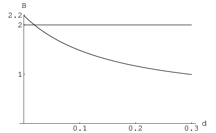
A search algorithm finds a local maximum for and returns the values of the free parameters. The function has a maximum of 2.19 with values , and . As expected, the Bell combination is most nonlocal when there is no noise present and the squeezed state is a pure two-mode squeezed state. In this case, one finds a stronger violation for large r and small intensity . To see how the internal noise affects the nonlocality of the state we set and let and vary in Fig.2.

It is clear that the diffusion parameter destroys the nonlocal features of the state. Fig. 3 shows a cross-section of the three dimensional graph of Fig. 2 for . The Bell combination is greater than 2 for small values of the diffusion parameter, . On a large scale, we find that as d increases the Bell combination decreases, reaches a minimum, and then increases to approach 2 from below.
V Continuous Variable Werner States
Using the two-mode squeezed state of Eq.(1), a class of nonseparable, non-Gaussian, mixed states can be explored. We will consider two cases: a convex combination of a pure entangled state with an uncorrelated mixed state, and a convex combination of a pure entangled state with a classically correlated state. The first case is the analogue of the Werner state for continuous variables.
Werner Werner 1989 investigated the state
| (30) |
for which is a convex combination of a maximally entangled state for finite dimension with a maximally mixed state obtained by a partial trace over the maximally entangled state. It was shown that such a state is nonseparable if and only if
| (31) |
V.1 Nonlocality of the continuous variable Werner state
A natural extension of a Werner state for infinite dimensions is a convex combination of a maximally entangled state with the maximally mixed state
| (32) |
for two modes of light, A and B. This state is analogous to the Werner state when the squeezing parameter r is infinite. The continuous variable phase-space representation of this state is given by
| (33) |
where is the marginal Wigner function obtained by the integration
| (34) |
over the variables of one mode. When r is infinite, the Wigner function is the EPR state and the function has infinite variance representing a maximally mixed state of knowledge. Note that Eq.(33) is not a Gaussian operator, but rather, it is a linear superposition of Gaussian operators. The separability conditions for a linear superposition of two Gaussian operators have not yet been established. However, it has been shown that the state is nonseparable if Mista 2002. This is the limit of the finite dimensional case, Eq.(31), as the dimension of the Hilbert space, d, approaches infinity.
A test of nonlocality for the state in phase space can be performed using the same Bell combination given by Eq.(28). It is found that the state remains nonlocal for a region of mixtures lying between and . Adding a mixed state to the entangled state rapidly degrades the nonlocal features.

V.2 Nonlocality of the phase-diffused state
In addition to the Werner state of Eq.(32) for continuous variables, a different convex combination has some interesting properties. Let us consider the state
| (35) |
which is a convex combination of a two-mode squeezed state with a phase-averaged state. Rather than integrating over one mode of light, an integration over the phases of both modes is performed. The state
| (36) |
describes phase diffusion of two light modes such that each mode has a completely random phase. The integral of Eq.(36) leads to a phase-averaged Wigner function given by
| (37) |
where is the modified Bessel function of the first kind. In contrast to the Werner state, this state does not factorize into a product of functions containing each mode. The state is a classically correlated state. The state of Eq.(35) now being considered is a mixture of a state containing quantum correlations and a state containing classical correlations. The nonlocality of this state is examined by considering an expansion for small intensity, , of the Bell combination given by Eq.(28). This expansion
| (38) |
reveals that the state (35) is nonlocal for all . This is seen in Fig.(5) which shows that only the case washes out the nonlocal features completely. Thus, we have presented a classically correlated state which, when mixed with even the smallest amount of a quantum correlated state, shows nonlocal features.

VI Conclusion
In this paper we examined the two-mode squeezed state with internal quantum noise. The Fokker-Planck equation was solved to obtain an exact solution for the Wigner function. The steady-state and nonsteady-state regimes were explored. We found that nonlocal features of this state exist in the regime where no steady-state solution exists.
The parameter space contains separable and nonseparable states, both mixed and pure. Only one pure state exists which is nonseparable. Nearly all states in the parameter space are mixed states. Using the Gaussian Wigner function for the state, the separability criterion was determined to identify those mixed states which are nonseparable. There exists a set of nonseparable mixed states for which the quantum diffusion can be large .
Using the Wigner function, a test of nonlocality in phase space determined the effect of internal quantum noise on Bell’s inequality. As expected, the noise parameters reduce the nonlocality of the state. But there is still a region of mixed entangled states which are nonlocal. To further study nonseparable mixed states exhibiting nonlocality, we investigated Werner-type states for continuous variables. We found that mixing the two-mode squeezed state with a product of two thermal states destroys the nonlocal features state. Additionally, we found that mixing the pure two-mode squeezed state with a phase-diffused, classically correlated state did not destroy the nonlocal features, regardless of the amount of mixing. With this, we have provided an example of a classically correlated state which, when mixed with even the smallest amount of pure entangled state, is nonlocal.
Acknowledgements.
This work was partially supported by a KBN grant No. 2PO3B 02123 and the European Commission through the Research Training Network QUEST.References
- Mandel (1995) L. Mandel and E. Wolf, Optical Coherence and Quantum Optics, (Cambridge University Press , (1995)).
- Aspect (1982) A. Aspect, P. Grangier and G. Roger, Phys. Rev. Lett., 49, 91 (1982).
- Banaszek (1998) K. Banaszek and K. Wdkiewicz, Phys. Rev. A, 58, 4345, (1998); K. Banaszek and K. Wdkiewicz, Phys. Rev. Lett., 82, 2009, (1999)
- Kheruntsyan (2000) K.V. Kheruntsyan and K.G. Petrosyan, Phys. Rev. A, 62, 015801, (2000).
- Kim (2000) H. Jeong, J. Lee and M.S. Kim, Phys. Rev. A, 61, 052101 (2000).
- Carmichael (1999) H.J. Carmichael, Statistical Methods in Quantum Optics 1: Master Equations and Fokker-Planck Equations, (Springer-Verlag, (1999)).
- Englert (2002) B.-G. Englert and K. Wdkiewicz, Phys. Rev. A, 65, 054303, (2002).
- Simon (2000) R. Simon, Phys. Rev. Lett., 84, 2726, (2000).
- Bell (1964) J.S. Bell, Physics, 1, 195, (1964); J.S. Bell, Rev. Mod. Phys., 38, 447, (1966) .
- Werner (1989) R.F. Werner, Phys. Rev. A, 40, 4277, (1989).
- Mista (2002) L. Mita, R. Filip, and J. Fiurek, Phys. Rev. A, 65, 062315, (2002).