Applications of Coherent Population Transfer to Quantum Information Processing
Abstract
We develop a theoretical framework for the exploration of quantum mechanical coherent population transfer phenomena, with the ultimate goal of constructing faithful models of devices for classical and quantum information processing applications. We begin by outlining a general formalism for weak-field quantum optics in the Schrödinger picture, and we include a general phenomenological representation of Lindblad decoherence mechanisms. We use this formalism to describe the interaction of a single stationary multilevel atom with one or more propagating classical or quantum laser fields, and we describe in detail several manifestations and applications of electromagnetically induced transparency. In addition to providing a clear description of the nonlinear optical characteristics of electromagnetically transparent systems that lead to “ultraslow light,” we verify that — in principle — a multi-particle atomic or molecular system could be used as either a low power optical switch or a quantum phase shifter. However, we demonstrate that the presence of significant dephasing effects on the metastable levels destroys the induced transparency. Finally, a detailed calculation of the relative quantum phase induced by a system of atoms on a superposition of spatially distinct Fock states predicts that a significant quasi-Kerr nonlinearity and a low entropy cannot be simultaneously achieved in the presence of arbitrary spontaneous emission rates. Within our model, we identify the constraints that need to be met for this system to act as a one-qubit and a two-qubit conditional phase gate.
I INTRODUCTION
I.1 Quantum Information Processing
With developments in theory and experiment over the last few years, there has been a dramatic growth of interest in the area of quantum information processing and communication.Lo et al. 1998; Bouwmeester et al. 2000; Nielsen and Chuang 2002 There are now strong indicators that this fundamental research field could lead to a whole new quantum information technology in the future. Working practical quantum cryptosystems exist already.Stucki et al. 2002; Gisin et al. 2002 It is known that large (many qubit) quantum computers, if they can be built, would be capable of performing certain tasks (such as factoring large composite integers or searching) much more efficiently than conventional classical computers. Rather smaller (tens or hundreds of qubits) quantum processors would be able to perform quantum simulations unreachable with any classical machine and such processors also have the potential to extend the working distances and applicability of quantum communications.
There are currently numerous possible routes for quantum computing hardware.Braunstein and Lo 2000; Clark 2001 Many of these are based on coherent condensed matter systems. While at present such systems generally exhibit less coherence than qubits based on fundamental entities (such as ions or atoms), the goals are to increase this sufficiently for error correction techniques to be applicable and to utilize the potential fabrication advantage to make condensed matter many-qubit processors. Even if this proves to be the way forward, it seems certain that there will be a need for separate quantum processors to communicate with each other in a quantum coherent manner. Coherent electromagnetic fields are likely the best candidates for realizing this goal. In addition, some quantum information processing may be performed directly on photon qubits, using non-linear Turchette et al. 1995 or linear quantum optical processes.Knill et al. 2001 So, photon qubits (or other quantum coherent states of the electromagnetic field) certainly have a number of important uses for quantum computing. However, they play center stage when it comes to communication, because the best way to send quantum information over large distances is certainly using light, either down optical fibers or even through free space.Stucki et al. 2002
Given all this, the study of coherent interactions between light and matter is an extremely important topic.Lukin and Imamoǧlu 2001; Monroe 2002 It is hard to see how large scale quantum information technology can emerge without the ability to easily interconvert traveling photon qubits and stationary matter qubits.DiVincenzo 1997; DiVincenzo 2000 Such interconversion would enable the construction of quantum networks Zoller et al. 1997, where communication between matter qubit nodes is mediated through photons. The ability to perform quantum gates (one- and two-qubit) directly on qubits encoded into photons is highly desirable for communication and computing. In addition, the coherent storage of photon qubits would open up new possibilities for quantum information processing.
Another very important application of quantum phenomena is to achieve tasks in classical (optical) information processing and communication. These applications will likely be the first to impact on future information technology. In this work we study aspects of coherent population transfer phenomena and discuss how the emergent effects may be applicable for producing large optical phase shifts and for switching. These effects in themselves are useful for conventional optical data processing. However, if in addition they can be demonstrated to work on non-classical input states of light, then they have the potential to form the basis of one- and two-qubit gates. We present a detailed calculation of the relative quantum phase induced by a system of atoms on a superposition of spatially distinct Fock states (a “dual rail” photon qubit) and identify the conditions under which this performs as a useful one-qubit phase gate. We also consider the qubit limit of one of the control fields applied to the system, and thus how a conditional two-qubit phase gate can be realized.
I.2 Electromagnetically Induced Transparency
The basic interaction between an atom and a photon is weak, which is why photons are so good for communication purposes. In order to enhance the interaction, one can either seek to use many actual atoms—an ensemble—or many “images” of a single atom, in effect created by the mirrors of a very high- cavity. The latter cavity QED approach has produced numerous impressive experimental and theoretical results over the last few years, Kimble 1998 but from the perspective of using atoms to manipulate light for information processing, we focus on the former ensemble approach.Lukin 2003
Photons, or light in general, can interact strongly with an ensemble of atoms, leading to a number of very interesting effects. The basis of many of these is the idea of electromagnetically induced transparency (EIT), a specific example of coherent population transfer.Harris 1997 Here, quantum interference can be used to effectively cancel the would-be absorption in an atomic medium, rendering it transparent. Ordinarily, a light signal on resonance with an atomic transition ( being the lower and long-lived level) interacts strongly with the atoms. However, if a third long-lived level comes into play and a control field resonant with is applied, the atoms are stimulated into states which cannot absorb,Arimondo 1997; Boller et al. 1991 and so in effect the atomic medium is transparent to the signal. These so-called “dark states” are coherent superpositions of and . We discuss this effect in detail for such three-level atoms. As will be seen, the transparency occurs only exactly on resonance. A transparency window, necessary for practical applications, can be opened by use of four-level atoms. Our focus in this work is the use of such EIT systems for the optical information processing applications. However, other important and interesting directions and applications exist, which can be followed up in detail elsewhere.
The intimate link between absorption and dispersion also means that EIT media can be used to manipulate the group velocity of light pulses.Harris et al. 1992 This can be reduced dramatically below the speed of light in vacuum through reducing the power in the control field and increasing the atomic density of the EIT medium. Various experiments demonstrated the potential of this effect, but the significant breakthrough came in 1999 when Hau et al. Hau et al. 1999 produced a group velocity of 17 m/s for light pulses in sodium vapor. Further developments continue to emerge. It is something of an oversimplification to regard a light pulse as simply slowing down as it propagates through an EIT medium. The strong interaction of the light with the atoms can effectively be diagonalized through the concept of quasiparticles (well known in condensed matter physics). In this case the propagation through the EIT system is described by quasiparticles called dark-state polaritons Fleischhauer and Lukin 2000, which are a coherent superposition of photons and spins. These polaritons move at a velocity given by the group velocity of their photonic component. An EIT system can therefore act as a ”delay line” for light pulses, an effect which in itself has significant application potential for communication. However, the ultimate limit of this effect is a complete slowing, leading to quantum memory for photons.Fleischhauer and Lukin 2002; Juzeliūnas and Carmichael 2002; Mewes and Fleischhauer 2002; Fleischhauer and Mewes 2001 As the (externally controllable) polariton group velocity is reduced towards zero, the photonic component of the polariton also reduces. In effect, the quantum state of the light field is stored in long-lived spin states of atoms within the EIT medium. This clearly has significant potential for quantum communication and information processing applications.
In a sense the whole scenario can also be reversed, with atomic ensembles (as opposed to the photons) being the principal information carriers, with interactions being controlled through electromagnetic fields. A number of novel quantum phenomena, also with potential for communication and processing applications, can arise in this case. It is possible to make quantum nondemolition measurements on the collective spin degree of freedom of atomic ensembles Kuzmich and Polzik 2000 using light. The interaction between such ensembles and light has also been employed to create a level of entanglement between the collective spin degrees of freedom of two atomic ensembles Julsgaard et al. 2001, a first step towards QIP with collective spins. Small ensembles of atoms can also exhibit analogous effects to the well known solid state mesoscopic phenomena such as Coulomb blockade. In very small capacitance sub-micron devices the strong Coulomb energy makes just a few energy levels relevant, and enables the manipulation of individual electronic charges. Likewise in small atomic ensembles the strong dipole-dipole interactions make just a few energy levels relevant, and it is possible to manipulate individual excitations of these spin systems and exhibit ”dipole blockade” phenomena.Lukin et al. 2001; Brennen et al. 1999; Jaksch et al. 2000; Lukin and Hemmer 2000
In this work we develop a theoretical framework for the exploration of quantum mechanical coherent population transfer phenomena, with a particular emphasis on the aspects of nonrelativistic quantum electrodynamics that play a strong role in potential classical and quantum information processing applications. We begin by outlining a general formalism for quantum optics in the Schrödinger picture, and we include a general phenomenological representation of Lindblad decoherence mechanisms. We use this formalism to describe the interaction of a single stationary multilevel atom with one or more propagating classical or quantum laser fields, assuming that this interaction is sufficiently weak that the population of the ground state is never significantly depleted. In addition to providing a clear description of the nonlinear optical characteristics of electromagnetically transparent systems that lead to “ultraslow light,” we verify that — in principle — a multi-particle atomic or molecular system could be used as either a low power optical switch or a quantum phase shifter. However, we demonstrate that the presence of significant dephasing effects destroys the induced transparency, and that increasing the number of particles weakly interacting with the probe field only reduces the nonlinearity further.
II REPRESENTATION OF THE ELECTROMAGNETIC FIELD
We wish to simplify our treatment of the quantum electromagnetic field as much as possible without introducing approximations which will result in significant disagreements with experimental results. Therefore, we begin our discussion of field quantization with the model of a unidirectionally propagating traveling wave shown in Fig. 1.Cohen-Tannoudji et al. 1992 As a result of the finite round-trip length of the cavity, the electromagnetic field is comprised of a superposition of discrete longitudinal modes with different wavevectors , angular frequencies , and polarization unit vectors , where , that satisfy the orthogonality condition . The field interacts with an ensemble of atoms located within the cavity; since the resonator is lossless, the only mechanism able to alter the number of photons in a given mode is the stimulated emission and absorption of photons in that mode.

In the laboratory, a typical experiment will most likely employ a continuously tunable multi-frequency traveling-wave field interacting with an atom in free space. Our model can represent such an experiment if two conditions are satisfied:Cohen-Tannoudji et al. 1992
- 1.
The resonator enforces an amplitude and local transverse spatial distribution on the model field that is identical to that of the experiment. Therefore, the exact number of photons in a given mode is not important when modeling a classical field, provided that the mean field intensity (approximately given by , where is the mean number of modes occupying the mode volume ) and mode shape are preserved.
- 2.
The cavity length is sufficiently long that the spontaneous emission spectrum of the atom is not altered.
In principle, we can model the tunability of the laser field by assuming that the positions of the resonator mirrors can be microscopically adjusted.
In the Schrödinger picture,11 1 In the Heisenberg picture, . we can represent the quantized transverse electric field operator as a discrete sum over the allowed wavevectors and possible polarizations :
| (1) |
where the dimensionless resonator eigenfunction describes the transverse spatial dependence of a field with a characteristic spot size , and satisfies both and the volume normalization condition
| (2) |
Therefore, the coefficient has the dimensions of an electric field.
We will apply the creation and annihilation operators and to the corresponding Fock (number) states through the ladder operator equationsLoudon 2000
| (3a) | |||||
| (3b) | |||||
The Fock state is an eigenstate of the unperturbed Hamiltonian22 2 Note that we have explicitly neglected the quantum electrodynamic contribution to the Hamiltonian from the vacuum.
| (4) |
with the eigenvalue , giving the total energy stored in photons of mode . In fact, we can ensure that we have chosen the correct value for the normalization constant by integrating the corresponding expectation value of the electromagnetic energy density over the mode volume. Applying Eq. (2), we obtain
| (5) |
as expected.
In this work, we will pass from the quantum regime to the classical limit through the coherent state ,Cohen-Tannoudji et al. 1992 defined in terms of the single-mode (i.e., single frequency and single polarization ) Fock states as
| (6) |
where is defined in terms of the mean occupation number as
| (7) |
Since is an eigenstate of the single-mode destruction operator with eigenvalue , we have
| (8a) | |||||
| (8b) | |||||
giving
| (9) |
where the associated classical field amplitude is
| (10) |
Therefore, for a given resonator mode containing exactly photons, we can associate the quantity with a classical field amplitude at . In practice, we will allow this classical amplitude — and therefore the mean photon number — to vary slowly in time when we study the adiabatic interaction of pump-probe pulses in our discussions of semiclassical coherent population transfer. However, we must be careful when passing from the quantum to the classical regime when the number of photons in a pulse is relatively small. In Section III.3, we show that weak coherent fields that are used to manipulate a quantum optical nonlinearity can be disrupted, in the sense that the field can no longer be represented as a coherent state after the interaction has ceased. In all cases, the atom + field system dynamics can be correctly described by tracking the evolution of individual energy (i.e., Fock) eigenstates, and then evaluating the sum given by Eq. (6) either analytically or numerically.
III ELECTROMAGNETICALLY INDUCED TRANSPARENCY
One of the most striking examples of coherent population transfer is electromagnetically induced transparency, where the absorption of a weak probe field by an atomic or molecular medium is mitigated by a second control field.Marangos 1998; Marangos 2000 In general, we will be concerned with systems that are weakly pumped, in the sense that we will assume that the perturbed atom(s) will remain primarily in the ground state.

III.1 Quantum Optics of the Two-Level Atom
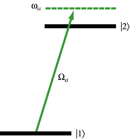
The electric dipole interaction between a two-level atom and a nearly resonant electromagnetic field is shown schematically in Fig. 2. In the semiclassical view of Fig. 2(a), the two atomic energy levels are separated by the energy , and coupled by a field oscillating at the angular frequency . However, in the quantum view of Fig. 2(b), the outer-product states of the atom + photons system separate into manifolds coupled internally by resonant transitions;Cohen-Tannoudji et al. 1992 if we define the detuning parameter
| (11) |
then the energy difference between the two levels of a given resonant manifold is far smaller than the difference between two adjacent manifolds.
Based on Fig. 2(b), we write the unperturbed Hamiltonian of the system in the Schrödinger pictureCohen-Tannoudji et al. 1977 as
| (12) |
where and are respectively the creation and annihilation operators for photons with energy and polarization vector , and are the atomic raising and lowering operators. Now, given an atom initially in the ground state and photons stored in the (lossless) resonator, the two eigenstates of the unperturbed Hamiltonian are and , with the eigenvalues
| (13) |
and
| (14) |
In the long-wavelength approximation, the electric dipole/field coupling interaction Hamiltonian for a single atom at is given explicitly byCohen-Tannoudji et al. 1989; Cohen-Tannoudji et al. 1992; Loudon 2000
| (15) |
In the basis of the unperturbed Schrödinger eigenstates, the matrix elements of the interaction Hamiltonian are
| (16) |
Therefore, if we define the effective coupling constant
| (17) |
and the effective Rabi frequency
| (18) |
then in the unperturbed Schrödinger basis
| (19) |
we obtain the total Hamiltonian
| (20) |
where we have subtracted from both diagonal terms. Note that we are using the bare eigenstates (rather than dressed statesCohen-Tannoudji et al. 1992) of the unperturbed Hamiltonian in the Schrödinger picture; the resulting perturbed Hamiltonian agrees with that of the corresponding semiclassical system in the interaction picture.
The evolution of the wavefunction
| (21) |
is governed by the Schrödinger equationCohen-Tannoudji et al. 1977
| (22) |
which has the formal solution
| (23) |
where the evolution operator is given by
| (24) |
and
| (25) |
Decoherence phenomena significantly complicate the evolution of the two-level manifold of Fig. 2(b). For example, spontaneous emission by the excited atom can scatter a photon into the free-space boundary volume (the “environment”) enclosing the idealized resonator of Fig. 1 at a rateCohen-Tannoudji et al. 1992
| (26) |
causing a transition from the the central manifold of Fig. 2(b) to the lower manifold. Strictly speaking, then, a completely general model describing incoherent population transfer phenomena must incorporate multiple manifolds. However, in this work, we are primarily concerned with applications of nonrelativistic quantum electrodynamics to quantum information processing, particularly high-fidelity quantum gate operations. In this case, the resonantly-coupled manifold of interest is ; therefore, spontaneous emission by the excited atom causes a transition from the product state to , a state lying in the lowest manifold. (In Section II, we explicitly assumed that the resonator of Fig. 1 does not modify the spontaneous emission spectrum, so we do not consider spontaneous emission into the cavity mode.) This transition effectively destroys the information carried by the quantum state of the electromagnetic field, and therefore a detailed analytical representation of the subsequent evolution of the state of the system is uninteresting. In practice, we can recover our resonant-coupling approximation by extending our product states to append an entry indicating whether a photon with frequency has been emitted into the environment, giving us a new single-photon basis, extended from Eq. (19) to
| (27) |
The introduction of decoherence into our model will prevent us from describing the two-level system state using the pure vector given by Eq. (21). Therefore, in the extended basis of Eq. (27), we introduce the corresponding density matrixCohen-Tannoudji et al. 1977 of the atom-photon system as
| (28) |
We can then use the corresponding total Hamiltonian
| (29) |
and an appropriate set of initial conditions to solve the density matrix equations of motionCohen-Tannoudji et al. 1977
| (30) |
where we have incorporated damping through the decoherence operator . We adopt the Lindblad formLindblad 1976; Nielsen and Chuang 2002 of , given by
| (31) |
to preserve both positive probabilities and a positive semidefinite density operator. The Lindblad operator represents a general dissipative process occurring at the rate . For example, we can describe the depopulation of the product state (due either to spontaneous emission from the atomic state to the environment , or to photon transmission or scattering losses in the cavity) at the rate using the lowering operator
| (32) |
and pure dephasing of the state at the rate using the operator
| (33) |
where is the identity matrix. For example, in the case , we have
| (34) |
and
| (35) |
Since we have assumed in Section II that the resonator of Fig. 1 does not modify the spontaneous emission spectrum of the atom, we have . Therefore, if we assume that atomic level is metastable and that the cavity is lossless, then we obtain the decoherence operator
| (36) |
where
| (37a) | |||||
| (37b) | |||||
| (37c) | |||||
| (37d) | |||||
We substitute Eq. (28), Eq. (29), and Eq. (36) into Eq. (30) to obtain
| (38a) | |||||
| (38b) | |||||
| (38c) | |||||
and then solve for the elements , , and using a “bootstrapping” method for the initial condition . If we assume that the interaction is unsaturated (i.e., ) so that for all , and that — to zeroth order in — varies slowly compared to , then will adiabatically follow and assume some quasi-steady-state value . Therefore, if we ignore short-term transients we must obtain
| (39) |
and subsequently from Eq. (38c)
| (40) |
where
| (41) |
Collecting results and solving for , we quickly find
| (42a) | |||||
| (42b) | |||||
| (42c) | |||||
where
| (43) |
and . Therefore, , and the quasi-steady-state density matrix describes a pure state only in the weak-field limit.
In the limit where the photon number is sufficiently small that , is a valid approximation for only when the time satisfies . It is worth noting that this steady state does not result if the system parameters are chosen so that the constraint is not strictly satisfied. In Fig. 3, we have plotted the real and imaginary parts of the off-diagonal density matrix element as a function of time for the case where . Even though , the magnitude of decays significantly on a time scale that is only a few times the transient lifetime. The characteristic time can be lengthened by increasing the detuning or by decreasing the Rabi frequency .


The expectation value of the microscopic polarization of the atom at is simply
| (44) |
where the first term arises from the annihilation process and the second from the creation process. We define the corresponding complex linear susceptibility in terms of the macroscopic polarization and the associated classical field amplitude using the expression
| (45) |
where is the effective mode volume given by Eq. (2). Therefore, we can calculate the complex susceptibility using the definition
| (46) |
which, after applying Eq. (17) and Eq. (18) to Eq. (41), gives
| (47) |
By convention, the real refractive index and the linear absorption coefficient are defined in terms of the real and imaginary parts of the susceptibility as
| (48a) | |||||
| (48b) | |||||
We have plotted the real and imaginary parts of Eq. (47) in Fig. 4, with units chosen so that . Note that the frequency with the largest dispersion (at ) corresponds to the frequency with the greatest absorption.


We can increase the susceptibility defined by Eq. (46) by increasing the number of atoms placed in the interaction region shown in Fig. 1. We assume that atoms are at rest near in a volume that is small compared to , where is the effective area of the fundamental laser mode at the beam waist, and is the Rayleigh length of the mode. Then, in a traveling-wave cavity, the Rabi frequency of each atom has a negligible spatial dependence, and is given by Eq. (18). In the unsaturated, weak-field case, the lower level of the quantum manifold shown in Fig. 2(b) has become -fold degenerate, since any one of the atoms can be excited to the upper atomic level via resonant excitation. We therefore define the unperturbed -atom basis
| (49) |
where the entry represents the -element string , describing all atoms in the ground state , and represents the same string, with the element at position replaced by a ‘2’, indicating that atom has been excited to the upper level . In this basis, we write the density matrix as
| (50) |
and, if we neglect any interactions between the atoms, the Hamiltonian as
| (51) |
We can construct the -atom Lindblad decoherence operator by allowing each atom to scatter an absorbed photon to the environment at the rate (independent of position), and we assume that the pure dephasing of the state occurs at the rate . If we repeat the single-atom quasi-steady-state approach that led to Eqs. (42), then in the limit in the noninteracting -atom case, we obtain
| (52a) | |||||
| (52b) | |||||
| (52c) | |||||
where Eqs. (52) have the same form as Eqs. (42) — independent of — but with the new time constant
| (53) |
Note that we have implicitly assumed that the population of the system ground state has not been significantly depleted (i.e., ).
Extending Eq. (44) to the -atom ensemble near , we obtain an expectation value of the microscopic polarization given by
| (54) |
where, in the quasi-steady-state regime where the time satisfies ,
| (55) |
Note that scales linearly with only in the weak-field limit where the probability that more than one atom has been excited to the upper level is negligible.
In Section IV.1, we will calculate both the quantum phase shift and the scattering rate encountered by a single photon optically coupled with one or more two-level atoms in the interaction region of the model resonator shown in Fig. 1. We can anticipate those results now using the definition of the complex susceptibility given by Eq. (46) in a semiclassical calculation. Suppose that our resonator encloses a coherent state with and contains atoms in an interaction region of length having the effective volume . Then we can approximate the total phase shift per round trip of the corresponding electromagnetic field as
| (56) |
where , and the fraction of the circulating electromagnetic power absorbed per round trip as
| (57) |
If we substitute Eq. (55) into Eq. (46), then we obtain the -atom susceptibility , and the corresponding refractive index change . If , then the round-trip time is given by , and we obtain for the corresponding classical electromagnetic field amplitude at
| (58) |
where the complex frequency shift is given by
| (59) |
or, after applying Eq. (46),
| (60) |
Therefore, in the classical linear-optical limit, the mean phase shift accumulated by the -photon coherent state at frequency after an elapsed time is
| (61) |
and the mean rate at which photons are absorbed and scattered by the atoms is, as expected,
| (62) |
where is given by Eq. (53). We see that — in the limit — this scattering rate is equivalent to , as expected from Eq. (38b). This semiclassical result is entirely consistent with that of the -atom quantum calculation found in Eq. (52), as predicted by extending Eq. (38a) to the -atom case.

III.2 Transparency of the Three-Level Atom
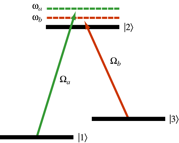
In Section III.1, we developed a formalism to describe the quantum optics of a two-level atom. In this formalism, the effective Rabi frequency represents the annihilation of a photon in mode , and is the diagonal element of corresponding to the (positively) detuned interaction between mode and the adjacent atomic transition in a given manifold of the energy-level diagram of the total system. In this section, we will follow the same formalism to analyze the quantum optical properties of the three-level atom shown in Fig. 5. Note that the upper atomic energy level and the new metastable level are coupled by a control field with angular frequency . It is the destructive quantum interference established by this control field that results in transparency (i.e., vanishing absorption) for the probe field at .
As in the case of the two-level atom, we reduce the semiclassical atomic system depicted in Fig. 5(a) to the quantum manifold given by Fig. 5(b). We will work in a manifold corresponding to an atom in state , with photons in mode and photons in mode . We again extend our basis to include energy dissipation to the environment by appending an entry to each product state, indicating the occurrence of scattering of a photon of frequency or . Therefore, the environment can be represented by the nonresonant submanifold that captures dissipated energy and preserves the trace of the density matrix. Referencing Section III.1, by inspection in the extended unperturbed Schrödinger basis
| (63) |
we obtain the total Hamiltonian
| (64) |
where we have defined the detuning parameter
| (65) |
the effective coupling constant
| (66) |
and the effective Rabi frequency
| (67) |
and we have subtracted the energy
from all diagonal terms.
The dynamics of a strongly-coupled system (e.g., a system having intracavity fields that are sufficiently intense that dephasing can be ignored) is often described using dressed states,Cohen-Tannoudji et al. 1992 where the submatrix of the Hamiltonian corresponding to the vectors and is diagonalized in the case of perfectly resonant tuning. For our purposes, weak fields and linearized (Lindblad) decoherence models generally allow the unperturbed eigenvectors to serve as a reasonably accurate basis set. For example, if we diagonalize the Hamiltonian given by Eq. (64) with , we find the nontrivial eigenvalues
| (68a) | |||||
| (68b) | |||||
| (68c) | |||||
where , and the nonzero eigenvectors
| (69a) | |||||
| (69b) | |||||
| (69c) | |||||
in the basis of Eq. (63). Therefore, if we assume that the system is entirely in the ground state at , we find
| (70) |
Therefore, in the strongly-coupled case, the population of the state is given by . We anticipate, then, that in a weakly coupled system with appreciable decoherence this population will remain small for all if and/or .
We now generalize the phenomenological discussion of decoherence presented in Section III.1 to describe more complex atomic energy-level schemes. We define as the total free-space depopulation rate to the environment of product state arising both from spontaneous emission from to all lower atomic levels and from transmission and scattering losses in the cavity, and as the pure dephasing rate for the state . In general, the decoherence coefficient of the term appearing in the Lindblad decoherence operator given by Eq. (31) can be quickly written down using a straightforward set of rules:
- 1.
In all cases, .
- 2.
If and , then
(71) - 3.
If and , then
(72) - 4.
If and , then
(73) - 5.
The value of the term corresponding to in is chosen to ensure that .
In the following analysis, we assume that atomic level is metastable so that . We substitute Eq. (64) and Eq. (31) into Eq. (30) and seek the quasi-steady-state solution in the unsaturated weak-field limit , assuming that and for all . Then we obtain , , (where ), and
| (74a) | |||||
| (74b) | |||||
with and , where is given by Eq. (37a) and
| (75) |
Since Eq. (38a) remains valid for the three-level atom + photons system, we can follow the same bootstrap procedure to obtain the approximate solution for given by Eq. (39), and
| (76a) | |||||
| (76b) | |||||
Therefore, the steady-state solutions given by Eqs. (74) are valid at any time where the laser parameters have been chosen to allow the inequality
| (77) |
to be satisfied.


Substituting Eq. (74a) into Eq. (46), we obtain the susceptibility (linear in )
| (78) |
When , the new detuning terms in Eq. (78) have remarkable implications for both the refractive index and the absorption coefficient given by Eq. (48). In Fig. 6, we assume that the control field has been tuned to the resonance frequency of the atomic transition so that , and we plot the real and imaginary parts of the complex susceptibility as a function of the normalized detuning for several values of the normalized control Rabi frequency . When , the absorption and dispersion curves reduce to those of the two-level atom shown in Fig. 4. However, when , near the absorption vanishes completely over a frequency range with a full width at half-maximum (FWHM) of
| (79) |
Over the same frequency range, the dispersion of the refractive index is proportional to , resulting in a significant increase in the group refractive index and a corresponding reduction in the group velocity at frequency . However, the dispersion cannot be made arbitrarily large by reducing the amplitude of the control field, because in the limit the width of the transparency window given by Eq. (79) becomes . Instead, the magnitude of the control field must be chosen to allow all significant spectral components of the probe pulse with carrier frequency to be transmitted with the maximum possible dispersion. (In an inhomogeneously broadened medium such as a dilute gas, only those atoms with Doppler-shifted resonance frequencies that are coincident with influence the group velocity of the probe beam.Javan et al. 2002; Lee et al. 2003)
Note that the transparency predicted by Eq. (74a) arises whenever , generating a pathway for a “virtual transition” between the unperturbed atomic energy levels and . In the steady-state case, the absorption by the atom of a photon of frequency never occurs, in the sense that a measurement of the state of the system will never find the atom in the level . Instead, the control field creates a coherent superposition of the and paths in Hilbert space such that destructive interference effectively reduces the transition rate to zero.
We can estimate the Rabi frequency resulting from a particular choice of experimental parameters by noting that both the spontaneous emission rate given by Eq. (26) and the Rabi frequency given by Eq. (18) depend on the electric dipole matrix element . If we assume that , then we find that
| (80) |
where is the resonant atomic absorption cross section at wavelength ,Cohen-Tannoudji et al. 1992 is the effective laser mode cross-sectional area, and is the free spectral range of the ring resonator. If we were simulating the adiabatic interaction of a pulsed laser field with a stationary atom, then would represent the bandwidth of the pulse profile function,Blow et al. 1990; van Enk and Fuchs 2002; Loudon 2000; Chan et al. 2002; Domokos et al. 2002 although more complex transients can arise when the interaction is non-adiabatic.Greentree et al. 2002a In the weak-control-pulse case where , we would require that for maximum transmission of the signal pulse at frequency . If, as an example, we choose , the Rabi frequency required to open a sufficiently large transparency window is
| (81) |
Assuming realistic optical focusing parameters, in free space the optimum value of the ratio is about 20% for Gaussian beams,van Enk and Kimble 2000; van Enk and Kimble 2001 but in waveguides it can approach unity.Domokos et al. 2002 If we neglect dephasing and set , then , and if the branching ratio is approximately unity. Therefore, in order to open the transparency window just wide enough to admit every photon in the probe pulse, we must have in free space, and about half that value in a waveguide. As an example, for interactions of single probe photons having with rubidium atoms (with a lifetime of level of 27 ns), the above parameters require , giving a FWHM of the transparency window of about 1 MHz. Therefore, only pulses with durations longer than 300 ns can safely propagate through the window.
The assumption that is generally valid in dilute gases, where decoherence arises primarily from spontaneous emission, although the introduction of Doppler broadening alters the frequency dependence of the susceptibility given by Eq. (78).Javan et al. 2002; Lee et al. 2003 The ultraslow group velocity of light propagating through an appropriately prepared gas sampleHau et al. 1999 can be reduced dynamically to zero, allowing probe pulses at frequency to be stored in the resulting atomic coherence and subsequently recovered after a controllable time delay.Phillips et al. 2001 Both transparency and storage of light has been demonstrated in a solid-state system (Pr:YSO) where cooling to liquid helium temperatures reduces the dephasing interactions between atomic levels and .Turukhin et al. 2002 However, in semiconductor-based systems, where the possibility that may be higher given the dependence of the off-diagonal decoherence rates on a common set of Lindblad parameters, these conclusions become less certain.Greentree et al. 2002b For example, in units where the absorption of the equivalent two-level system (corresponding to ) is 1, the absorption coefficient of the general three-level system at is given by
| (82) |
Hence, if we assume that and , we obtain an absorption coefficient that is 50% of the corresponding two-level value, and the system is no longer transparent. Similarly, the dispersion of the general three-level system is
| (83) |
indicating that we must have to maintain a positive dispersion and a reduced group velocity for the probe field. For , the optimum value of the control Rabi frequency yielding the largest dispersion is given by when , resulting in a dispersion that is reduced by a factor of four relative to the case .
If we follow the approach of Section III.1 and extend our single-atom three-level analysis to include atoms, we draw essentially the same conclusion as in the two-level case: the susceptibility is enhanced by a factor of in the unsaturated, weak-probe-field limit. Adopting the notation of Section III.1, in the unperturbed basis
| (84) |
we have the -atom Hamiltonian
| (85) |
As in the case of noninteracting two-level atoms, the off-diagonal density-matrix elements for each atom are given by Eqs. (74), and Eq. (54) holds in the three-level case, with as before. The aggregate susceptibility is enhanced by a factor of only if the conditions and are satisfied; otherwise, when and , the transparency window is completely destroyed and the susceptibility reduces to that of two-level atoms. However, when these conditions are met, the absorption coefficient approaches zero as , and the group refractive index is increased by a factor of . This property allows us to compensate for the need to open a sufficiently large window to allow a pulse to propagate through the interaction region without significant loss by increasing the number of atoms in that region.
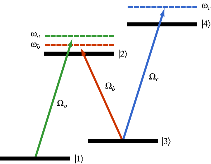
III.3 Tunable Transparency of the Four-Level Atom
The capability to transmit a particular probe field with very high fidelity and extraordinarily slow group velocity is enabled by the inclusion of the second control field in Fig. 5. However, since the probe frequency providing the greatest transparency results in a differential refractive index that is precisely zero, this system cannot be used to generate a significant relative phase shift. More precise deterministic control of the phase and intensity of the probe pulse can be obtained by adding the third field shown in Fig. 7, coupling the metastable atomic energy level with the upper energy level . As in the previous sections, we reduce the semiclassical atomic system depicted in Fig. 7(a) to the quantum manifold given by Fig. 7(b), and we will work in a manifold corresponding to an atom initially in state , with photons in mode , photons in mode , and photons in mode . We again extend our basis to include energy dissipation to the environment by appending an entry to each product state, indicating the occurrence of scattering of a photon of frequency , , or . Therefore, the environment should be represented by a nonresonant sub-manifold that captures dissipated energy and preserves the trace of the density matrix, resulting in the unperturbed Schrödinger basis
| (86) |

Referencing Section III.2, by inspection we then obtain the total Hamiltonian
| (87) |
where we have defined the detuning parameter
| (88) |
the effective coupling constant
| (89) |
and the effective Rabi frequency
| (90) |
and subtracted the energy
from all diagonal terms.
Again, we follow the general decoherence conventions established in Section III.2 to enumerate contributions to the decoherence operator using Eq. (31). We define as the total free-space depopulation rate to the environment of state and as the corresponding pure dephasing rate. We substitute Eq. (87) and Eq. (31) into Eq. (30) and seek the quasi-steady-state solution in the unsaturated weak-field limit , assuming that , , and for all . We neglect all contributions to density matrix elements of order and higher, and we obtain , , , (where ), and
| (91a) | |||||
| (91b) | |||||
| (91c) | |||||
where the remaining off-diagonal density matrix elements are (), is given by Eq. (37a), is given by Eq. (75), and is defined as
| (92) |
Since Eq. (38a) remains valid for the four-level atom + photons system, we can follow the same bootstrap procedure to obtain the approximate solution for given by Eq. (39), and
| (93) |
where . As in the three-level case, the steady-state solutions given by Eqs. (91) are valid at any time where the laser parameters have been chosen to allow the inequality
| (94) |
to be satisfied.
We see immediately that Eq. (91a) reduces to Eq. (74a) if . Therefore, in this limit the four-level system of Fig. 7 remains at least approximately transparent. However, in general, the absorption and dispersion curves shown in Fig. 6 can be significantly modified by a nonvanishing radiative coupling between the atomic states and . For example, when all coupling fields are resonantly tuned to the corresponding transitions (i.e., ), we have
| (95) |
Since the complex part of is related to the absorption coefficient by Eq. (48), we see that we have lost perfect transparency when the frequency is resonant, even if . However, the presence of the fourth atomic level and the corresponding nearly resonant electromagnetic field with frequency introduces an extremely large Kerr-like nonlinearity even at relatively low light intensities.Lukin and Imamoǧlu 2001; Harris et al. 1990; Schmidt and Imamoǧlu 1996; Imamoǧlu et al. 1997; Harris and Hau 1999; Rebić et al. 2002a; Rebić et al. 2002b; Braje et al. 2003 In particular, we can demonstrate that the four-level system of Fig. 7 can behave as either a low-energy quantum switchHarris and Yamamoto 1998; Yan et al. 2001a; Yan et al. 2001b; Braje et al. 2003 or a quantum phase-shifter,Schmidt and Imamoǧlu 1996 properties which can be harnessed for both classical and quantum information processing and distribution.Monroe 2002; Vitali et al. 2000; Lukin and Imamoǧlu 2000; Lukin et al. 2001; Fleischhauer and Mewes 2001; Fleischhauer and Lukin 2002
We assume that the magnitude of the Rabi frequency satisfies the inequality , so that we can define a complex third-order susceptibility for the transition by analogy with Eq. (45) as
| (96) |
where is the three-level linear susceptibility given by Eq. (78). If we expand in a power series about , we obtain
| (97) |
As in Section III.2, we set , we choose the values of (consistent with weak fields), and for simplicity we select . In Fig. 8 we plot the real and imaginary parts of the total susceptibility as a function of for three values of the relative detuning . As we discussed above, when , the probe field at will be strongly absorbed, and when transparency is largely restored, but there is a nonzero contribution to the refractive index at . We can see these effects more clearly by setting in Eq. (97) and then varying , as is done in Fig. 9. We note that when , the presence of a photon at (i.e., ) closes a “quantum switch” that causes the absorption of the probe photon,Harris and Yamamoto 1998; Yan et al. 2001a; Yan et al. 2001b and when , the atom acts as a “quantum phase shifter” that is largely transparent but shifts the relative phase of the probe photon.Schmidt and Imamoǧlu 1996 We explore the latter property of the four-level system in the next section, where we explicitly calculate the corresponding applied phase shift of a coherent superposition of single-photon states.


Following the approach of Section III.2, an extension of the single-atom four-level model to include atoms in the interaction region reveals that the susceptibility is enhanced by a factor of only in the unsaturated, weak-probe-field limit. Again adopting the notation of Section III.1, in the unperturbed basis
| (98) |
we have the -atom Hamiltonian
| (99) |
As in the case of noninteracting two-level and three-level atoms, the off- diagonal density-matrix elements for each atom are given by Eqs. (91), and Eq. (54) holds in the four-level case, with as before. The aggregate susceptibility is enhanced by a factor of only if and .
Our discussions have emphasized that the resonant nonrelativistic quantum electrodynamic interaction of the four-level system of Fig. 7 results in the generation of a giant third-order optical nonlinearity, commonly described as a Kerr nonlinearity in the literature.Lukin and Imamoǧlu 2001; Harris et al. 1990; Schmidt and Imamoǧlu 1996; Imamoǧlu et al. 1997; Harris and Hau 1999; Rebić et al. 2002a; Rebić et al. 2002b; Braje et al. 2003; Wang et al. 2001 Strictly speaking, an effective Kerr Hamiltonian with the form
| (100) |
causes the Fock state to evolve as
| (101) |
where . Therefore, if the evolution of the four-level system shown in Fig. 7 exhibits this Kerr behavior, then we can claim that the corresponding nonlinearity is in fact a Kerr nonlinearity. However, at low light levels, if one of the optical transitions is driven by a weak coherent state (rather than a Fock state), we can show that the structure of this nonlinearity is not strictly of the Kerr type unless . We begin by assuming that all dephasing rates are zero, and by solving the Schrödinger equation for the basis set given by Eq. (86) under the influence of spontaneous emission only. Using our adiabatic bootstrap approach, we find for the case that the -atom ground state evolves as
| (102) |
where
| (103) |
and . Note that when the inequality
| (104) |
is satisfied (equivalent to the assumption in the simple case where ), the probability that a single photon with frequency will be scattered by the atom becomes vanishingly small. Therefore, the evolution of the atomic ground state during a prolonged interaction with the compound Fock state will be governed primarily by the real part of Eq. (103); since and , the evolution of Eq. (102) has the Kerr form of Eq. (101) with the nonlinear coefficient
| (105) |
where the vacuum Rabi frequencies are given by .
Let us now replace the -photon Fock state with a coherent state parameterized by and assess the evolution of the corresponding unperturbed ground state
| (106) |
Since each unperturbed eigenstate evolves according to Eq. (102), after a time we find
| (107) |
where and
| (108) |
Note that is not a coherent state unless , for which . In Fig. 10, we have used Eqs. (106)–(107) to numerically evaluate the inner product for several values of the net phase shift , assuming that and . Note that for large phase shifts the inner product differs significantly from unity even when ; in fact, for , only if . Therefore, only when the coupling field driving mode closely approximates a classical field does EIT provide a true cross-Kerr nonlinearity.
Nevertheless, we can appreciate the magnitude of the optical Kerr nonlinearity even at low light levels by estimating the parameters included in Eq. (108). Let us assume that , and compute the phase shift induced by a system of 1000 non-interacting atoms in the case where . Using Eq. (80) as a guide, we estimate , and we assume a unit branching ratio for spontaneous emission from atomic level so that . If we let the Fourier-limited pulse duration be , then after the pulse has interacted with the atoms we obtain a phase shift of approximately 0.1 radians. This shift is about seventeen orders of magnitude larger than the corresponding value provided by a standard Kerr cell.Boyd 1999; Kok et al. 2003

IV QUANTUM INFORMATION PROCESSING
We wish to assess the utility of coherent population transfer for the creation, transmission, reception, storage, and processing of quantum information. In particular, we must evaluate the time dependence of coherent superpositions of discrete states of the atom + photon field that are (at least in principle) easily distinguished by direct detection of a photon with energy . For example, consider a system that is initially in a pure state consisting of a superposition of two manifold states, such as
| (109) |
where
- 1.
represents the atom in the ground state and zero photons in the resonator of Fig. 1; and
- 2.
represents the atom in the ground state and photons in the resonator.
If we subsequently apply the unitary phase shift operator to , then we obtain the result
| (110) |
where we note that each Fock photon contributes equally to the total accumulated phase. Similarly, if we begin with a superposition of an empty resonator and a coherent state , we find
| (111) |
in accordance with our intuition for classical fields. A simple physical implementation of such a dual-rail coherent superposition could be provided by the Mach-Zehnder interferometer shown in Fig. 11. In one arm of the interferometer, the single four-level atom represented by Fig. 7 is prepared using to provide a phase shift at the probe frequency while remaining largely transparent and dispersive. In the second arm, , and the system is tuned to match the absorption and dispersion provided by the atom in the first arm, allowing the interferometer to remain time-synchronous. In principle, we can simply use the real and complex parts of the susceptibilities given by Eq. (78) and Eq. (97) to determine the classical absorption and group velocity reduction provided by each system, as is done in standard treatments.Lo et al. 1998; Bouwmeester et al. 2000; Nielsen and Chuang 2002 In practice, however, we must be careful to demonstrate that the interaction of either arm with a photon at the probe frequency that has entered the interferometer at the input port will entangle the quantum mechanical paths of that photon with each other but not with either of the atoms.

In this section, we solve the density matrix equation of motion given by Eq. (30) for product states that include the additional kets enumerated above, and we seek expressions for density matrix elements that allow us to directly read out the phase in Eq. (110) and Eq. (111) in terms of experimentally determined parameters such as Rabi frequencies and laser detunings. We will discover that constraints must be placed on possible values of these parameters in systems suffering from decoherence because of the necessity of maintaining either high fidelity (or low entropy) in systems without active quantum error correction, or (equivalently) high data rates in corrected systems.
IV.1 The Two-Level Atom
Following the example of the dual-rail state introduced in Eq. (109), we wish to further extend the basis of Eq. (27) to include the possibility that all photons have followed another quantum trajectory, and are not found in the interaction region containing the two-level atom(s). We add one element, and one state vector, to include the atomic variables and the environment in Eq. (109):
| (112) |
Now we can rewrite the two-level density matrix given by Eq. (28) in this basis as
| (113) |
We can then use the corresponding total Hamiltonian
| (114) |
to solve for the density matrix element . We include in our model the same phenomenological decoherence mechanisms introduced in Section III.1, and we do not introduce new dephasing processes between the superposed loaded and unloaded resonators.
At , we assume that the system is in the pure state superposition
| (115) |
and we wish to identify a later time (if possible) where the system state vector has evolved to the pure state
| (116) |
i.e., a state where both the atomic state and the environment can be factored out of the Hilbert space, leaving a nonzero relative phase difference between the remaining basis vectors. At each of these times, the density matrix will have the form
| (117) |
where establishes the initial condition.
In the absence of decoherence, the nonzero density matrix elements are quickly found to be
| (118a) | |||||
| (118b) | |||||
| (118c) | |||||
| (118d) | |||||
| (118e) | |||||
where is given by Eq. (25). It is clear that has the form given by Eq. (117) at the times , where is a nonnegative integer. At these times, the argument of is given by
| (119) |
where we have chosen the sign of to be consistent with that of the argument of when is small. When the system is undamped, a field with the detuning
| (120) |
acquires a relative phase of at the time
| (121) |
Therefore, for a given value of applied to an undamped atomic system, a resonantly tuned field with and obtains a phase shift earliest.
In the presence of decoherence, we seek the quasi-steady-state solution to the density matrix equation of motion defined by Eq. (30), now emphasizing the single matrix element . We build the Lindblad decoherence matrix operator by applying Eq. (31) to the new density matrix Eq. (113), and we extract the system of coupled linear differential equations
| (122a) | |||||
| (122b) | |||||
where the decoherence constants are
| (123a) | |||||
| (123b) | |||||
Using the bootstrap method described in Section III.1, we solve Eqs. (122) for the element with the initial conditions and . If we again assume that the interaction is unsaturated (i.e., ) so that for all , and that — to zeroth order in — varies slowly compared to , then Eqs. (122) yields the approximate solution
| (124) |
where
| (125) |
It is straightforward to extend Eq. (124) to include a coherent unsaturated interaction with independent atoms localized within a volume that is small compared to at . We begin by extending both the -atom density matrix and Hamiltonian given by Eq. (50) and Eq. (51), respectively, to include the coherent superposition with the empty resonator, as was done in Eq. (113) and Eq. (114). We find that Eq. (124) remains unchanged if we make the substitution and , so that—in the low-dephasing limit, after the transient terms in Eq. (124) have decayed—the effect of the placement of atoms in the interaction region is to replace the time with . In this limit, Eq. (124) and Eq. (125) are entirely consistent with Eq. (58) and Eq. (60), except for the appearance of the photon number in the denominator of Eq. (60). Since Eq. (125) was obtained using an -photon Fock state (rather than a coherent state, as was implicitly used in the semiclassical estimate of ), we expect an additional factor of from the analysis leading to Eq. (110).
In the unsaturated limit, our analysis of the conditions required to obtain a particular phase shift is significantly different from that of the undamped case. Clearly, if we wish to accumulate a large phase shift before the system state has become significantly mixed, the resonant detuning should satisfy the inequality
| (126) |
This constraint can only be met in the weak-field case if the dephasing rate between the upper and lower atomic energy levels is small enough that . In this limit, dephasing can be neglected, and the argument of the density matrix element is given approximately by the undamped value
| (127) |
or, at time ,
| (128) |
At time , Eq. (124) gives for the magnitude of
| (129) |
Now, in order to achieve a phase shift of , we must choose a long delay time such that , giving and
| (130) |
It is clear that we must detune the laser field such that so that we can minimize the effects of decoherence, but it is not obvious how to choose a specific value of . First, we can define the fidelity (a measure of distance between quantum states) of two density matrices and asNielsen and Chuang 2002
| (131) |
or, in the case of a pure state and an arbitrary state ,
| (132) |
Applying Eq. (132) to the density matrix given by Eq. (113) and the pure state
we obtain
| (133) |
Second, we can compute the entropy of using the definitionNielsen and Chuang 2002
| (134) |
where the sum is carried over the nonzero eigenvalues of . Now, the density matrix elements and are proportional to , while is proportional to . Therefore, by Eq. (126), we ignore these terms in the density matrix given by Eq. (113), and we apply Eq. (134) in the limit to obtain
| (135) |
In principle, we can choose the value of to obtain particular values of the entropy and fidelity, and then — in an -atom system — allow the system to evolve until time to accumulate a phase shift. In practice, in many cases the probe field frequency cannot be modified post hoc, particularly in applications where a phase shift other than is required and/or more than one type of atom or molecule is placed in consecutive interaction regions.
It is already clear from Eq. (135) and Eq. (133) that we must have if we wish to hold and (base 2) for quantum information purposes. If, as an example, we also have , then after a time we will obtain a linear phase shift of . However, if we require and , then we must have and wait until a time to obtain a linear phase shift of . In other words, even though we are using a large detuning, requirements of small entropy and high fidelity imply that we will need either extraordinarily long interaction times or many identical noninteracting atoms to achieve nontrivial phase shifts.
IV.2 The Four-Level Atom
A calculation of the real and imaginary parts of in the case of the four-level atom proceeds in essentially the same fashion as the corresponding calculation for the two-level case described in the previous section. Again we further extend the product state basis given by Eq. (86) to include a “second rail” as an alternative quantum path for the probe photons, corresponding to a density matrix and Hamiltonian (extended from Eq. (87) as Eq. (114) was from Eq. (29)). The matrix elements , , , and are mutually coupled, and we seek an approximate solution using the bootstrap method used in previous sections. We neglect transient (homogeneous) solutions to the coupled ODEs, and we assume that is much larger than the magnitudes of the other three elements. Under these conditions, in the unsaturated limit we obtain the quasi-steady-state solution
| (136) |
where
| (137) |
and are given by Eq. (123), and
| (138a) | |||||
| (138b) | |||||
If we set to minimize absorption, and if the dephasing rates are much smaller than the depopulation rates of the upper atomic levels, then Eq. (137) becomes
| (139a) | |||||
| (139b) | |||||
where
| (140a) | |||||
| (140b) | |||||
Note that Eq. (139b) has precisely the same form as the corresponding two-level result given by Eq. (125). Hence, the nonlinear phase shift derived from Eq. (139b) can be as large as the corresponding linear phase shift obtained from Eq. (125), indicating the presence of an enormous third-order nonlinearity that couples the three fields.Schmidt and Imamoǧlu 1996; Nielsen and Chuang 2002; Vitali et al. 2000; Wang et al. 2001 In principle, this nonlinearity requires only modest detunings to provide both a high differential phase shift and a low absorption rate in the semiclassical realm.
However, in the quantum information processing applications described above, we must also check that the photon-atom system is effectively disentangled when the dipole interaction is switched off. In the limit , the earliest elapsed time required to obtain a phase shift of and the corresponding fidelity and entropy are respectively given by
| (141) | |||||
| (142) | |||||
| (143) |
Given a sufficiently long interaction time, it is clear from Eq. (140a) that a large phase shift can be accumulated using a relatively small net detuning even when represents the Hamiltonian matrix element describing the dipole interaction of a single photon with a single atom.Shimizu et al. 2002 However, the value of needed to maintain a high fidelity and a low entropy depends on other system parameters. For example, in the limitSchmidt and Imamoǧlu 1996
| (144) |
we note that we must have to achieve and . Hence, relatively large detunings are still required when the four-level system is used for quantum information processing applications. However, in the limit where the spontaneous emission rate of atomic state in Fig. 7 has been strongly suppressed,
| (145) |
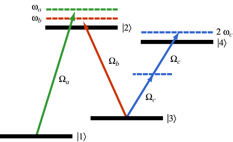
we find from Eq. (142) and Eq. (143) that , a constraint that can be satisfied easily for small detunings whenever . Suppression of spontaneous emission from level can be achieved in at least two different ways. First, the interaction region can be placed within a photonic bandgap crystal (PBC) designed so that photons with frequency must be injected through a defect in the crystal structure. Second, a different atomic system could be chosen with an energy level structure similar to that shown in Fig. 12, where the final dipole transition in Fig. 7(a) has been replaced by a two-photon transition to the metastable atomic level . Although the details of the calculations leading to Eq. (139b) will certainly change for this system, the relative weakness of the two-photon transition amplitude can be effectively offset by a suitably smaller choice of the value of the detuning frequency .
If the controlled coupling transition is driven by a Fock state, then the four-level atom + field system provides a large cross-Kerr nonlinearity of the form when the constraint given by Eq. (145) is satisfied. Neglecting the imaginary part of Eqs. (139), we find that the evolution corresponds to that of the Kerr Hamiltonian given by Eq. (101), with the nonlinear coefficient given by Eq. (105). In this case, the entanglement of the atoms and fields is negligible, and the fidelity of the final state is high. However, if the coupling transition is driven by a coherent state, then — as shown in Fig. 10 — the electromagnetic intensity of that state (i.e., the magnitude of the Poynting vector) must be quite large to ensure that the atoms and fields are completely disentangled at the conclusion of the gate operation. This condition requires that , reducing the magnitude of the effective cross-Kerr nonlinearity given by Eq. (108).
We have demonstrated so far that it is possible to apply an arbitrary phase shift to an initial state of a photonic qubit tuned to the transition in Fig. 7, resulting in the final state . Clearly it is straightforward to perform Hadamard gates on qubits encoded in photons in this manner, through use of simple linear optics (beamsplitters). With the tuneable EIT phase shift gate, the required range of single qubit gates needed for universal quantum information processing is therefore covered. The other necessary ingredient for universal quantum processing DiVincenzo 1995; Lloyd 1995; Barenco et al. 1995; Nielsen and Chuang 2002 is a two qubit entangling gate. For photonic qubits which generally interact very weakly with each other, this is the more difficult gate to realize. One solution is to use measurement and feedback to create an effective strong non-linearity between photonic qubits.Knill et al. 2001 However, it is clearly of real significance for photonic quantum information processing to consider the possibility of a direct non-linear coupling between photonic qubits using an EIT system, to realize, for example, a conditional two-qubit phase gate.
Consider a case (depicted schematically in Fig. 13) with two photon number encoded qubits (target and control), where the target qubit is tuned to the transition frequency and the control qubit is tuned to the transition frequency of Fig. 7, so this mode is now a quantum rather than classical control field. As shown above, if no photon is present in the transition, then the target qubit acquires no phase shift. However, if a photon with frequency is present in the transition, then the target qubit evolves to . Hence, this system implements a conditional phase shift and is extremely useful for quantum information processing. In fact, for a conditional phase shift of the operation provides a universal two-qubit gate capable of maximally entangling two initially unentangled photonic qubits. The input product state can be transformed to the maximally entangled state , as shown schematically in Fig. 13. Therefore, in principle, universal optical quantum information processing can be performed with such EIT systems.

To illustrate this we consider the error probability in generating the conditional phase shift on the amplitude. Fig. 14 shows the error probability in generating the phase-shifted amplitude for single photons in the and modes of the four-level system, as a function of the average photon number in the coherent drive applied to mode , for various values of the chosen phase shift. Clearly as long as the applied drive in mode is pushed towards being a classical field and so the EIT system provides an accurate cross-Kerr nonlinearity, the amplitude can in principle receive a large and accurate phase shift. The dependence of the nonlinearity on the various parameters is given in Eq. (108). From Fig. 14 we see that the gate requires a drive field with a large , but from Eq. (108) this reduces the strength of the nonlinearity, which increases the value of required for the chosen phase shift (for a given detuning). So, as discussed in Section IV.1 and Section IV.2, it is crucial that the effects of decoherence are kept small, in particular the spontaneous emission from level , in order to perform a two-qubit gate with small error. Detailed analysis of the effects of decoherence on the EIT phase gates will be addressed in future work.

Clearly the conditional phase shift can be put to good use in other quantum processing applications. One extremely useful device is a high efficiency non-demolition detector for photons. If instead of a single photon state on the transition, a weak coherent state is input, a measurable (by standard techniques) phase shift arises conditional on the single-photon Fock amplitude of a qubit in the transition. In effect a projective measurement in the computational basis can be performed on the photonic qubit, with the qubit being available for re-use afterwards rather than being absorbed. This can be achieved with high efficiency () and with just a few hundred atoms in the EIT system. Details of this detector are reported elsewhere.Munro et al. 2003
V CONCLUSIONS
In Section III.3, we demonstrated that it should be possible to use the four-level atomic system of Fig. 7 as the foundation for both a (so-called) quantum switch and a phase-shifter. For example, the quantum switch is, in principle, simple to implement: given the availability of a photon with frequency , if a photon with frequency is present (i.e., ), then a probe photon with frequency will be absorbed; otherwise, if , then the probe photon will be transmitted. All this shows that conventional classical information processing operations are possible on optical data—single bit phase shifts and conditional (two-bit) switching. These effects have significant potential for applications to conventional optical communications.
In Section IV, we demonstrated that it should be possible to operate the four-level atomic system as a “dual rail” photon qubit phase shifter, provided that the spontaneous emission from the atomic level can be suppressed. The size of the phase shift and the fidelity of the gate are quantified in terms of the system parameters in our model, so the trade-off between the size of the phase shift, the accuracy of the gate, the time of operation and the atomic and control parameters can be analyzed in detail. A single photon phase gate, coupled with others that can be performed using linear optical elements, enables the performance of arbitrary single qubit operations. Universal quantum information processing requires the addition of a suitable entangling two-qubit gate.DiVincenzo 1995; Lloyd 1995; Barenco et al. 1995; Nielsen and Chuang 2002 We have also demonstrated that in principle, the phase shifter arrangement can be turned into such a gate—a two-qubit conditional phase gate—by using a qubit input also on the control field at frequency . Therefore such EIT systems can in principle be used to enable universal quantum information processing with “dual rail” photon qubits. Coupled with ideas such as quantum memory for photons Fleischhauer and Lukin 2002; Juzeliūnas and Carmichael 2002; Mewes and Fleischhauer 2002; Fleischhauer and Mewes 2001 and non-absorbing photon detectors,Munro et al. 2003 it is clear that EIT systems present a very promising route forward for few-qubit quantum information processing.
Indeed, given the experimental progress with EIT phenomena over the last few years, it seems likely that these QIP applications can tested and developed over the next few years. Of course, more detailed research still needs to be done. For example, further refinements to our model to include coherent wavepacket representations of the fields are needed to realistically assess in detail the performance of the two-qubit gate. This will be addressed in future work.
Acknowledgements.
We thank Kae Nemoto and Pieter Kok for helpful conversations, and Adrian Kent and Sandu Popescu for numerous detailed suggestions after carefully reading the manuscript.References
- Lo et al. (1998) H.-K. Lo, S. Popescu, and T. Spiller, eds., Introduction to Quantum Computation and Information (World Scientific Publishing, Singapore, 1998).
- Bouwmeester et al. (2000) D. Bouwmeester, A. Ekert, and A. Zeilinger, eds., The Physics of Quantum Information (Springer-Verlag, Berlin, 2000).
- Nielsen and Chuang (2002) M. A. Nielsen and I. L. Chuang, Quantum Computation and Quantum Computation (Cambridge University Press, Cambridge, 2002).
- Stucki et al. (2002) D. Stucki, N. Gisin, O. Guinnard, G. Ribordy, and H. Zbinden, New J. Phys. 4, 41.1 (2002).
- Gisin et al. (2002) N. Gisin, G. Ribordy, W. Tittel, and H. Zbinden, Rev. Mod. Phys. 74, 145 (2002).
- Braunstein and Lo (2000) S. Braunstein and H.-K. Lo, eds., Experimental Proposals for Quantum Computation, vol. 48 of Fortschr. Phys. (2000), number 9–11.
- Clark (2001) R. G. Clark, Experimental Implementation of Quantum Computation (Rinton Press, Princeton, 2001).
- Turchette et al. (1995) Q. A. Turchette, C. J. Hood, W. Lange, H. Mabuchi, and H. J. Kimble, Phys. Rev. Lett. 75, 4710 (1995).
- Knill et al. (2001) E. Knill, R. Laflamme, and G. J. Milburn, Nature 409, 46 (2001).
- Lukin and Imamoǧlu (2001) M. D. Lukin and A. Imamoǧlu, Nature 413, 273 (2001).
- Monroe (2002) C. Monroe, Nature 416, 238 (2002).
- DiVincenzo (1997) D. P. DiVincenzo, in Mesoscopic Electron Transport, edited by L. Kowenhoven, G. Schön, and L. Sohn (Kluwer Academic Publishers, Dordrecht, 1997), NATO ASI Series E.
- DiVincenzo (2000) D. P. DiVincenzo, Fortschr. Phys. 48, 771 (2000).
- Zoller et al. (1997) J. I. C. P. Zoller, H. J. Kimble, and H. Mabuchi, Phys. Rev. Lett. 78, 3221 (1997).
- Kimble (1998) H. J. Kimble, Phys. Scr. T76, 127 (1998).
- Lukin (2003) M. D. Lukin, Rev. Mod. Phys. 75, 457 (2003).
- Harris (1997) S. E. Harris, Phys. Today 50, 36 (1997).
- Arimondo (1997) E. Arimondo, in Progress in Optics, edited by E. Wolf (North-Holland, Amsterdam, 1997), vol. 35, pp. 259–354.
- Boller et al. (1991) K.-J. Boller, A. Imamoǧlu, and S. E. Harris, Phys. Rev. Lett. 66, 2593 (1991).
- Harris et al. (1992) S. E. Harris, J. E. Field, and A. Kasapi, Phys. Rev. A 46, R29 (1992).
- Hau et al. (1999) L. V. Hau, S. E. Harris, Z. Dutton, and C. H. Behroozi, Nature 397, 594 (1999).
- Fleischhauer and Lukin (2000) M. Fleischhauer and M. D. Lukin, Phys. Rev. Lett. 84, 5094 (2000).
- Fleischhauer and Lukin (2002) M. Fleischhauer and M. D. Lukin, Phys. Rev. A 65, 022314 (2002).
- Juzeliūnas and Carmichael (2002) G. Juzeliūnas and H. J. Carmichael, Phys. Rev. A 65, 021601 (2002).
- Mewes and Fleischhauer (2002) C. Mewes and M. Fleischhauer, Phys. Rev. A 66, 033820 (2002).
- Fleischhauer and Mewes (2001) M. Fleischhauer and C. Mewes (2001), eprint arXiv:quant-ph/0110056.
- Kuzmich and Polzik (2000) A. Kuzmich and E. S. Polzik, Phys. Rev. Lett. 85, 5639 (2000).
- Julsgaard et al. (2001) B. Julsgaard, A. Kozhekin, and E. S. Polzik, Nature 413, 400 (2001).
- Lukin et al. (2001) M. D. Lukin, M. Fleischhauer, R. Cote, L. M. Duan, D. Jaksch, J. I. Cirac, and P. Zoller, Phys. Rev. Lett. 87, 037901 (2001).
- Brennen et al. (1999) G. K. Brennen, C. M. Caves, P. S. Jessen, and I. H. Deutsch, Phys. Rev. Lett. 82, 1060 (1999).
- Jaksch et al. (2000) D. Jaksch, J. I. Cirac, P. Zoller, S. L. Rolston, R. Côté, and M. D. Lukin, Phys. Rev. Lett. 85, 2208 (2000).
- Lukin and Hemmer (2000) M. D. Lukin and P. R. Hemmer, Phys. Rev. Lett. 84, 2818 (2000).
- Cohen-Tannoudji et al. (1992) C. Cohen-Tannoudji, J. Dupont-Roc, and G. Grynberg, Atom-Photon Interactions: Basic Processes and Applications (John Wiley & Sons, New York, 1992).
- Loudon (2000) R. Loudon, The Quantum Theory of Light (Oxford University Press, Oxford, 2000), 3rd ed.
- Marangos (1998) J. P. Marangos, J. Mod. Opt. 45, 471 (1998).
- Marangos (2000) J. P. Marangos, Nature 406, 243 (2000).
- Cohen-Tannoudji et al. (1977) C. Cohen-Tannoudji, B. Diu, and F. Laloë, Quantum Mechanics, vol. 1–2 (John Wiley & Sons, New York, 1977).
- Cohen-Tannoudji et al. (1989) C. Cohen-Tannoudji, J. Dupont-Roc, and G. Grynberg, Photons and Atoms: Introduction to Quantum Electrodynamics (John Wiley & Sons, New York, 1989).
- Lindblad (1976) G. Lindblad, Comm. Math. Phys. 48, 119 (1976).
- Javan et al. (2002) A. Javan, O. Kocharovskaya, H. Lee, and M. O. Scully, Phys. Rev. A 66, 013805 (2002).
- Lee et al. (2003) H. Lee, Y. Rostovtsev, C. J. Bednar, and A. Javan, Applied Physics B: Lasers and Optics 33–39, 119 (2003).
- Blow et al. (1990) K. J. Blow, R. Loudon, S. J. D. Phoenix, and T. J. Shepherd, Phys. Rev. A 42, 4102 (1990).
- van Enk and Fuchs (2002) S. J. van Enk and C. A. Fuchs, Phys. Rev. Lett. 88, 027902 (2002).
- Chan et al. (2002) K. W. Chan, C. K. Law, and J. H. Eberly, Phys. Rev. Lett. 88, 100402 (2002).
- Domokos et al. (2002) P. Domokos, P. Horak, and H. Ritsch, Phys. Rev. A 65, 033832 (2002).
- Greentree et al. (2002a) A. D. Greentree, T. B. Smith, S. R. de Echaniz, A. V. Durrant, J. P. Marangos, D. M. Segal, and J. A. Vaccaro, Phys. Rev. A 65, 053802 (2002a).
- van Enk and Kimble (2000) S. J. van Enk and H. J. Kimble, Phys. Rev. A 61, 051802(R) (2000).
- van Enk and Kimble (2001) S. J. van Enk and H. J. Kimble, Phys. Rev. A 63, 023809 (2001).
- Phillips et al. (2001) D. F. Phillips, A. Fleischhauer, A. Mair, R. L. Walsworth, and M. D. Lukin, Phys. Rev. Lett. 86, 783 (2001).
- Turukhin et al. (2002) A. V. Turukhin, V. S. Sudarshanam, M. S. Shahriar, J. A. Musser, B. S. Ham, and P. R. Hemmer, Phys. Rev. Lett. 88, 023602 (2002).
- Greentree et al. (2002b) A. D. Greentree, D. Richards, J. A. Vaccaro, A. V. Durrant, S. R. de Echaniz, D. M. Segal, and J. P. Marangos, Phys. Rev. A 65, 023818 (2002b).
- Harris et al. (1990) S. E. Harris, J. E. Field, and A. Imamoǧlu, Phys. Rev. Lett. 64, 1107 (1990).
- Schmidt and Imamoǧlu (1996) H. Schmidt and A. Imamoǧlu, Opt. Lett. 21, 1936 (1996).
- Imamoǧlu et al. (1997) A. Imamoǧlu, H. Schmidt, G. Woods, and M. Deutsch, Phys. Rev. Lett. 79, 1467 (1997).
- Harris and Hau (1999) S. E. Harris and L. V. Hau, Phys. Rev. Lett. 82, 4611 (1999).
- Rebić et al. (2002a) S. Rebić, A. S. Parkins, and S. M. Tan, Phys. Rev. A 65, 043806 (2002a).
- Rebić et al. (2002b) S. Rebić, A. S. Parkins, and S. M. Tan, Phys. Rev. A 65, 063804 (2002b).
- Braje et al. (2003) D. A. Braje, V. Balić, G. Y. Yin, and S. E. Harris (2003), eprint arXiv:quant-ph/0309084.
- Harris and Yamamoto (1998) S. E. Harris and Y. Yamamoto, Phys. Rev. Lett. 81, 3611 (1998).
- Yan et al. (2001a) M. Yan, E. G. Rickey, and Y. Zhu, Opt. Lett. 26, 548 (2001a).
- Yan et al. (2001b) M. Yan, E. G. Rickey, and Y. Zhu, Phys. Rev. A 64, 041801 (2001b).
- Vitali et al. (2000) D. Vitali, M. Fortunato, and P. Tombesi, Phys. Rev. Lett. 85, 445 (2000).
- Lukin and Imamoǧlu (2000) M. D. Lukin and A. Imamoǧlu, Phys. Rev. Lett. 84, 1419 (2000).
- Wang et al. (2001) H. Wang, D. Goorsky, and M. Xiao, Phys. Rev. Lett. 87, 073601 (2001).
- Boyd (1999) R. W. Boyd, J. Mod. Opt. 46, 367 (1999).
- Kok et al. (2003) P. Kok, H. Lee, and J. P. Dowling, Phys. Rev. A 66, 063814 (2003).
- Shimizu et al. (2002) Y. Shimizu, N. Shiokawa, N. Yamamoto, M. Kozuma, and T. Kuga, Phys. Rev. Lett. 89, 223001 (2002).
- DiVincenzo (1995) D. P. DiVincenzo, Phys. Rev. A 51, 1015 (1995).
- Lloyd (1995) S. Lloyd, Phys. Rev. Lett. 75, 346 (1995).
- Barenco et al. (1995) A. Barenco, C. H. Bennett, R. Cleve, D. P. DiVincenzo, N. Margolus, P. Shor, T. Sleator, J. A. Smolin, and H. Weinfurter, Phys. Rev. A 52, 3457 (1995).
- Munro et al. (2003) W. J. Munro, K. Nemoto, R. G. Beausoleil, and T. P. Spiller (2003), eprint arXiv:quant-ph/0310066.