Topological Quantum Gates with Quantum DotsJournal: J. Opt. B: Quantum Semiclass. Opt.(special issue on Quantum Computing)
Abstract
We present an idealized model involving interacting quantum dots that can support both the dynamical and geometrical forms of quantum computation. We show that by employing a structure similar to the one used in the Aharonov-Bohm effect we can construct a topological two-qubit phase-gate that is to a large degree independent of the exact values of the control parameters and therefore resilient to control errors. The main components of the setup are realizable with present technology.
pacs
03.67.Lx,73.23.Hk1 Introduction
A very promising scenario for the implementation of quantum computation is considered to be the solid state realization of quantum dots [1, 2, 3]. The solid state arena is attractive because there is a great deal of technological knowledge already accumulated from the domain of classical computation. However, if we are to use solid state devices for quantum computation, we need to manipulate individual quantum systems, like electrons in quantum dots, that demand a much higher degree of control accuracy than currently available. There has been a number of recent proposals to address the issue of controlability by using geometrical and topological effects [4, 5]. The key advantage of these methods is that the resulting geometrical and topological gates do not depend on the overall time of the evolution, nor on small deformations in the control parameters. Possible manifestations of geometrical phases are the Berry phases obtained, for example, through a cyclic adiabatic evolution of a system [6] or through the Aharonov-Bohm effect [7]. Within solid state physics, there have even been proposals to implement Berry phases with Josephson Junctions [8] as well as Aharonov-Bohm phases encoded in the different spin states of electrons manipulated in quantum dot structures [9, 10].
In this paper we present a simple solid state implementation of a charge based structure that is capable of supporting both dynamical and geometrical quantum computation. Consider quantum dots that can either be empty or can accommodate an electron. In an array of quantum dots we assume that we are able to lower the potential between any two dots and facilitate the quantum tunneling between them. Intrinsically, the Hamiltonian of this system is governed mainly by three parts, namely the potential wall of height separating two successive dots, the Coulomb interaction between two electrons which is active when they are occupying the same dot or adjacent dots in a close proximity and the external laser fields which, in principle, can facilitate to move an electron along specific paths.
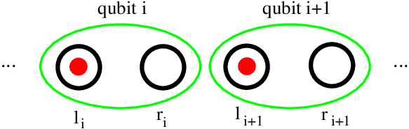
Imagine that we have an array of paired dots and that to each pair corresponds an electron as in Fig. 1. We can interpret the qubit to be encoded by the pair of dots ; if the electron is in the left dot () it corresponds to the logical state , while when it is in the right dot () this corresponds to the state . Preparation of the initial qubit state as well as the final read out are technically easy tasks. The performance of one qubit gates is achieved by lowering the potential wall between the pair of the dots and, hence, quantum tunneling between the two dots will create superpositions of the logical states [12] giving, for example, the state . Thus, any possible one qubit rotation can in principle be performed.
For a two-qubit phase-gate we need to perform a controlled transition where the state of one of the qubits is changed conditional on the state of the second qubit. We shall present in Section 2 three different ways of performing such a gate in a dynamical, geometrical and topological fashion. A controlled phase-gate can then allow us to execute any arbitrary quantum computation providing that we can also implement single qubit gates. Finally, in Section 3, a set of different potential implementations are presented based on current solid state technology.
2 Two qubit phase-gates
As we have seen the charge based quantum computation model consists of two dots and and an electron which can be in a state that is a superposition of occupying both of them. Indeed, if the electron is in the left dot then the state of the system can be represented as , where is the occupation number of dot , while if the electron is in the right dot then the state is written as . These states correspond to the logical and qubit states. How such a system can support entangling gates between the qubits is described in the following.
2.1 Dynamical phase-gate
In the purely dynamical implementation of the controlled phase-gate we rely on the fact that when two electrons are trapped in the neighboring wells, then their dynamical phase due to the Coulomb interaction is larger than when the electrons are far apart. Hence, when the dots are in the state , their extra phase with respect to all the other states is equal to , where is the increase in the electron energy due to the Coulomb repulsion and is the time during which the electrons are close enough to exhibit a non-negligible interaction. The evolution of the system of the two qubits in the basis , , and is then given by
After time we obtain a dynamical version of the two-qubit phase-gate. This gate is, in fact, algorithmically equivalent to the controlled-not gate and is capable of generating entanglement between two initially disentangled qubits. Most of the current proposals for implementation of quantum computation are based on dynamical gates.
2.2 Geometrical phase-gate
Now we would like to show how to implement the same gate in the same setting, but using the geometrical instead of the dynamical phase. Consider a homogeneous magnetic field in the neighborhood of the dots that comprise the logical array of qubits. An electron which spans a closed trajectory (loop) inside the magnetic field will acquire a phase factor proportional to the flux of the magnetic field encircled by the loop [7]. The electron can be moved around by applying an additional external time dependent laser field that guides the electron along the desired trajectory on a plane perpendicular to the magnetic field .

In the case of the controlled interaction we want to achieve, we can imagine that we encourage a cyclic evolution of an electron from the dot towards the dot of the second pair of dots as seen in Fig. 2. If there is no electron in the dot , then the loop of the first electron spans a surface given by and it is determined only by our controlled procedure since the electrons are non-interacting. As a result, after the first electron has returned to dot , it has acquired a phase given by . On the other hand, if there is an electron in dot then the trajectory of the first electron will be influenced by the additional Coulomb interaction (repulsion) and it will span a loop that encloses a smaller surface area . Hence, when the electron has returned to dot , then it has acquired a phase given by . It is clear that no non-trivial evolution will occur if the electron of the first qubit is in dot . The unitary evolution that is finally implemented in this way is of the form
which, up to a local phase rotation of qubit , is equivalent to a controlled phase-gate that changes only the state to the state . This is the geometrical version of a two qubit gate which was previously implemented dynamically.
2.3 Topological phase-gate
We notice that if there is a small change in the geometry of the loop in the previous evolution, then the form of the phase-gate will also change. This is a drawback of the previous model as, in general, the external field guiding the electron will fluctuate and therefore the acquired phase, which is proportional to the encircled magnetic flux due to the motion of the electron, will also suffer from this error in our control. We can remedy this problem by spatially restricting the magnetic field in the Aharonov-Bohm effect. The gate we now describe will be independent of the actual shape of the electron trajectory to a high degree. To achieve this, we need to place between each pair of dots a small solenoid with a large density magnetic field confined inside it [11] as depicted in Fig. 2. The control procedure of the gate is the same as the one presented in the geometrical case, only that now the solenoid is positioned inside the surface area . This is the surface which is not covered by the electron of qubit if and only if the electron of qubit is in the dot . The net effect resulting from this procedure is an evolution in the computational basis of the two qubits given by
where is proportional to the magnetic flux confined by the solenoid. In other words, by employing the Coulomb interaction it is possible for electron to acquire a fixed phase if it circulates around the solenoid, while no phase is obtained if the electron does not circulate around it. The phase is independent of the exact shape of the electron’s trajectory. This is, therefore, the topological version of the quantum phase-gate discussed before. Unlike the previous gates, it has the advantage that any deformation of the trajectory of the electron that does not alter its winding number around the solenoid has no effect whatsoever on the gate. Consequently, this offers us a high degree of independence from control errors.
3 Solid state implementation
The realization of the topological gate requires the confinement of the magnetic field to the very small area of the solenoid which is placed in-between the dots. We would like now to estimate how small the radius of the solenoid should be in order to compare it with the experimental state of the art. For simplicity we assume that the electron is confined in a one dimensional harmonic potential , where is the electron mass, is the trapping frequency and is the displacement of the electron. Consider the case where we want to move an electron from dot (see Fig. 2) towards dot positioned at , by displacing the trapping potential. If there is no electron in then the trapping potential carrying the electron from dot moves so that its final minimum is positioned at . If the electron exists at , then the final position of the traveling electron is determined by the minimum of the combined trapping potential and the Coulomb repulsion. An approximate estimate of the displacement of the new minimum is given by
| (1) |
Typical trapping frequencies are in-between and which results in in-between and . This distance is roughly the size of the region in which the magnetic field has to be confined in order to implement the topological evolution. The present technology [11] allows us to construct a solenoid with the dimensions smaller than , which is more than sufficient for the implementation of our proposal.
So far in our proposal the electron from dot has to continuously move from its original position to close to the other electron and then back to . However this does not need to be continuous as the electron can, in fact, perform the same looping trajectory by discrete tunneling between, for example three different dots.

Towards that direction, let us consider the implementation of the two qubit phase-gate as presented in the previous analysis, but with the configuration of four dots arranged as in Fig. 3. Consider a magnetic field , that is large enough so that the spins in the dots are aligned along the magnetic field, and henceforth play no role in the subsequent evolution. Assume a double dot system where is the Coulomb repulsion with single occupancy of each dot in the double dot system while at the same time no tunneling occurs between them. Allowing in addition the tunneling process to take place between neighboring dots, the resulting Hamiltonian of the system is given by
| (2) |
where
| (3) |
where is the annihilation operator of the electrons in the dot , is its free energy, is the tunneling coupling between the neighboring dots and and indicates nearest neighbors. Assume that the tunneling couplings can be turned on and off at will, obtaining the maximum value , and we shall assume for simplicity that is also the Coulomb potential for two electrons within the same dot. If dot is occupied, then the effective tunneling between and or and is . We shall consider the limit of large where we are in the Coulomb blockade regime, i.e. and hence, in that case, actual tunneling does not occur. In that case it is impossible to circulate an electron initially in the dot around the dots , , and back to if there is an electron in the dot , by turning on successively the couplings , and for time to transit the electrons from one dot to the other. On the other hand, if the dot is empty, an electron can go around the closed path acquiring a phase due to the Aharonov-Bohm effect. The latter is given by where is the area of the triangle spanned by the dots , and . In order to guarantee that the electron initially in will return back to its initial position if there is an electron in we have to activate , then again (the electron returns back in the case it is still in due to Coulomb blockade) and then . While is activated, the electron in does not move again due to the Coulomb blockade. Hence, at the end of this evolution the system returns back to the qubit states where there is no occupancy in the dots or . The resulting two-qubit gate is exactly the same as given in the previous section with the phase given by . Alternatively, the magnetic field can be confined in a solenoid imbedded in-between the dots , and . Therefore, this simple and realistic systems offers a possibility to implement the topological based quantum computation discussed at a more abstract level in Section .
Discussion and Conclusions
We have presented here three possible implementation of quantum gates. Every subsequent implementation, although more difficult to implement, offers a higher degree of reliability with respect to control errors. In the topological implementation, if the magnetic field is confined to a very small region of space between the quantum dots, we can achieve an arbitrary high fidelity of gate implementation. We even saw from a very simple analysis in the previous section that this is, in principle, possible with current technology. However, our analysis does not take into account other possible sources of errors, such as decoherence due to the coupling of the electron with the environment. The environment can, for example, act as a projective measurement determining the position of the electron thereby destroying any superposition of the electron occupancy states of different dots. Alternatively, the environment can destroy the phase coherence between different element of the superposition. For the particular analysis of the behaviour of geometric phases under classical and quantum noises see, for example, [14]. To successfully compensate this kind of errors, in parallel to the methods presented here, we will, most likely, have to resort to other existing methods like quantum error correcting codes [15] or error avoiding methods like in decoherence-free subspaces [16]. Note finally that we can interpret our structure as generating a single electron circulating current (vortex) by the electron in dot conditional on the presence of an electron in . This is a very interesting physical system in its own right that could be potentially used for other applications of quantum circuits, for example in measuring the flux of the magnetic field by the resulting relative phase between the two distinct possible evolutions. A similar model with three potential wells has also been used to describe generation of vortices in trapped Bose-condensates [17]. An elaborated analysis of our proposal including various decoherence mechanisms is therefore very much worthwhile and will be presented elsewhere.
References
References
- [1] D. Loss and D. P. DiVincenzo, Phys. Rev. A 57, 120 (1998); see also the review D. P. DiVincenzo et. al., Quantum Mesoscopic Phenomena and Mesoscopic Devices in Microelectronics, eds. I. O. Kulik and R. Ellialtioglu (NATO Advanced Study Institute, Turkey, 1999).
- [2] G. Burkard, D. Loss and D. P. DiVincenzo, Phys. Rev. B 59, 2070 (1999).
- [3] A. Ardavan et. al., “Nanoscale Solid State Quantum Computing”, to appear in Phil. Trans. R. Soc. London A (2003).
- [4] A. Kitaev, quant-ph/9707021.
- [5] J. Pachos, Phys. Rev. A 66, 042318 (2002).
- [6] M. V. Berry, Proc. Roy. Soc. London Ser. A 392, 45 (1984).
- [7] Y. Aharonov and D. Bohm, Phys. Rev. 115, 485 (1959).
- [8] G. Falci et. al., Nature 407, 355 (2000).
- [9] H. Akera, Phys. Rev. B 47, 6835 (1993).
- [10] D. Loss and E. V. Sukhorukov, Phys. Rev. Lett. 84, 1035 (2000); E. V. Sukhorukov and D. Loss, cond-mat/0106307 (2001).
- [11] H. D. Chopra and S. Z. Hua, Phys. Rev. B 66, 020403(R) (2002).
- [12] N. H. Bonadeo et. al., Science 282, 1473 (1998).
- [13] P. Solinas et. al., quant-ph/0301089 (2003).
- [14] A. Vourdas, Phys. Rev. A 64, 053814 (2001); A. Carollo et. al. quant-ph/0301037 (2003).
- [15] A. Steane, Nature 399, 124 (1999).
- [16] A. Beige et. al., Phys. Rev. Lett. 85, 1762-1765 (2000); see also L. Viola et. al., Science 293, 2059 (2001).
- [17] K. Nemoto et. al., Phys. Rev. A 63, 013604 (2001).