Quantum Communication Through an Unmodulated Spin Chain

Transmitting a quantum state (known or unknown) from one place to another is often an important task bennett00. It is required, for example, to link several small quantum processors for large-scale quantum computing. Thus it is very important to have physical systems which can serve as channels for quantum communication. We can either directly transmit a state through the channel, or we can first use the channel to share entanglement with a separated party and then use this entanglement for teleportation bennett93. The ideal channel for long distance quantum communications is an optical fiber. This requires interfacing a quantum computer (such as arrays of spins or ions) with optics. For short distance communications (say between adjacent quantum processors), alternatives to interfacing different kinds of physical systems are highly desirable and have been proposed, for example, for ion traps wineland02. In this letter, I propose a scheme to use a spin chain (a 1D magnet – real or simulated) as a channel for short distance quantum communication. The communication is achieved by placing a spin encoding the state at one end of the chain and waiting for a specific amount of time to let this state propagate to the other end (as shown in Fig.1(a)). This helps to avoid interfacing because both quantum computers and quantum channels can then be made by the same physical systems. Moreover, neither does the spin chain channel require the ability to switch interactions ”on” and ”off” (often a problem in quantum computer implementations zhou; benjamin), nor does it require any modulation by external fields (essential for quantum computation). This simplicity in comparison to a quantum computer makes it an ideal connector between quantum computers and realizable well before a quantum computer.

I will first present the scheme in a general setting for arbitrary graphs of spins with ferromagnetic Heisenberg interactions and later proceed to the realizable case of an open ended chain. Consider the general graph shown in Fig.1(b), where the vertices are spins and the edges connect spins which interact. Say there are $N$ spins in the graph and these are numbered $1,2,...,N$. The Hamiltonian is given by

$\vec{\sigma}^{i}=(\sigma_{x}^{i},\sigma_{y}^{i},\sigma_{z}^{i})$ in which $\sigma_{x/y/z}^{i}$ are the Pauli matrices for the $i$th spin, $B_{i}>0$ are static magnetic fields and $J_{ij}>0$ are coupling strengths, and $<i,j>$ represents pairs of spins. ${\bf H}_{\bf G}$ describes an arbitrary ferromagnet with isotropic Heisenberg interactions. We now assume that the state sender Alice is located closest to the $s$th (sender) spin and the state receiver Bob is located closest to the $r$th (receiver) spin (these spins are shown in Fig.1(b)). All the other spins will be called channel spins. It is also assumed that the sender and receiver spins are detachable from the chain. In order to transfer an unknown state to Bob, Alice replaces the existing sender spin with a spin encoding the state to be transferred. After waiting for a specific amount of time, the unknown state placed by Alice travels to the receiver spin with some fidelity. Bob then picks up the receiver spin to obtain a state close to the the state Alice wanted to transfer. As we never require individual access or individual modulation of the channel spins in our protocol, they can be constituents of rigid 1D magnets.

We assume that initially the system is initially cooled to its ground state $|{\bf 0}\rangle=|000...0\rangle$ where $|0\rangle$ denotes the spin down state (i.e., spin aligned along $-z$ direction) of a spin. This is shown for a 1D chain in the upper part of Fig.1(a). I will set the ground state energy $E_{0}=0$ (i.e., redefine ${\bf H}_{\bf G}$ as $E_{0}+{\bf H}_{\bf G}$) for the rest of this paper. We also introduce the class of states $|{\bf j}\rangle=|00...010....0\rangle$ (where ${\bf j}={\bf 1},{\bf 2},..{\bf s},..{\bf r},..,{\bf N}$) in which the spin at the $j$th site has been flipped to the $|1\rangle$ state. To start the protocol, Alice places a spin in the unknown state$|\psi_{in}\rangle=\cos{(\theta/2)}|0\rangle+e^{i\phi}\sin{(\theta/2)}|1\rangle$ at the $s$th site in the spin chain. We can describe the state of the whole chain at this instant (time $t=0$) as

Bob wants to retrieve this state, or a state as close to it as possible, from the $r$th site of the graph. Then he has to wait for a specific time till the initial state $|\Psi(0)\rangle$ evolves to a final state which is as close as possible to $\cos{\frac{\theta}{2}}|{\bf 0}\rangle+e^{i\phi}\sin{\frac{\theta}{2}}|{\bf r}\rangle$. As $[{\bf H}_{\bf G},\sum_{i=1}^{N}\sigma_{z}^{i}]=0$, the state $|{\bf s}\rangle$ only evolves to states $|{\bf j}\rangle$ and the evolution of the spin-graph (with $\hbar=1$) is

The state of the $r$th spin will, in general, be a mixed state, and can be obtained by tracing off the states of all other spins from $|\Psi(t)\rangle$. This evolves with time as

with

where $P(t)=\cos^{2}{\frac{\theta}{2}}+\sin^{2}{\frac{\theta}{2}}|f^{N}_{r,s}(t)|^{2}$ and $f^{N}_{r,s}(t)=\langle{\bf r}|\exp{\{-i{\bf H}_{\bf G}t\}}|{\bf s}\rangle$. Note that $f^{N}_{r,s}(t)$ is just the transition amplitude of an excitation (the $|1\rangle$ state) from the $s$th to the $r$th site of a graph of $N$ spins.

Now suppose it is decided that Bob will pick up the $r$th spin (and hence complete the communication protocol) at a predetermined time $t=t_{0}$. The fidelity of quantum communication through the channel averaged over all pure input states $|\psi_{in}\rangle$ in the Bloch-sphere ($(1/4\pi)\int\langle\psi_{in}|\rho_{out}(t_{0})|\psi_{in}\rangle d\Omega$) is then

where $\gamma=\arg\{f^{N}_{r,s}(t_{0})\}$. To maximize the above average fidelity, we must choose the magnetic fields $B_{i}$ such that $\gamma$ is a multiple of $2\pi$. Assuming this special choice of magnetic field value (which can always be made for any given $t_{0}$) to be a part of our protocol, we can simply replace $f^{N}_{r,s}(t_{0})$ by $|f^{N}_{N,1}(t_{0})|$ in Eq.(5). The spin chain then acts as an amplitude damping quantum channel preskill-notes; nielsen-book. It converts the input state $\rho_{in}=|\psi_{in}\rangle\langle\psi_{in}|$ to $\rho_{out}=M_{0}\rho_{in}M_{0}^{\dagger}+M_{1}\rho_{in}M_{1}^{\dagger}$ with the operators $M_{0}$ and $M_{1}$ (Kraus operators preskill-notes) given by

Now consider the transmission of the state of one member of a pair of particles in the entangled state $|\psi^{+}\rangle=\frac{1}{\sqrt{2}}(|01\rangle+|10\rangle)$ through the channel. This is the usual procedure for sharing entanglement between separated parties which precedes teleportation bennett00. The output state $\rho_{out}(t_{0})=\sum_{i=0,1}I\otimes M_{i}|\psi^{+}\rangle\langle\psi^{+}|I\otimes M_{i}^{\dagger}$ is

The entanglement ${\cal E}$ of the above state, as measured by the concurrence wootters is given by

Thus, for any non-zero $f^{N}_{r,s}(t_{0})$ (however small), some entanglement can be shared through the channel. This entanglement, being that of a $2\times 2$ system, can also be distilled horodecki into pure singlets and used for teleportation. Later we will estimate $f^{N}_{r,s}(t_{0})$ for very long open chains and show that entanglement can be distributed to arbitrary distances.

Eqs.(6) and (8) are exceptionally simple formulas for the fidelity of quantum communications and the entanglement shared through our spin-graph channel in terms of single transition amplitude $f^{N}_{r,s}(t_{0})$. We note here that such simple formulas, with slight modifications, will hold for spin-graphs with much wider class of interactions, as long as the state $|{\bf 0}\rangle$ does not evolve nielsen1.

We will now consider a linear open ended spin chain (Fig.1(a)), which is the most natural geometry for a channel. To use an analytically solvable Hamiltonian ${\bf H}_{\bf L}$ we assume $J_{ij}=(J/2)\delta_{i+1,j}$ (nearest neighbor interactions of equal strength) and $B_{i}=B$ (uniform magnetic field) for all $i$ and $j$ in Eq.(1) for ${\bf H}_{\bf G}$. The eigenstates of ${\bf H}_{\bf L}$, relevant to our problem are

where $m=1,2,...,N$, $a_{1}=1/\sqrt{N}$ and $a_{m\neq 1}=\sqrt{2/N}$ with energy (on setting $E_{0}=0$) given by $E_{m}=2B+2J(1-\cos\{{\frac{\pi}{N}(m-1)}\})$. In this case, $f^{N}_{r,s}(t_{0})$ is given by

where, $v_{m}=a_{m}\cos{\{\frac{\pi}{2N}(m-1)(2r-1)\}}e^{-iE_{m}t_{0}}$ and $IDCT_{s}(v_{m})=\sum_{m=1}^{N}a_{m}v_{m}\cos{\{\frac{\pi}{2N}(m-1)(2s-1)\}}$ is the $s$th element of the inverse discrete cosine transform of the vector $\{v_{m}\}$.

We now want to study the performance of our protocol for various chain lengths $N$ with $s=1$ and $r=N$ (Alice and Bob at opposite ends of the chain as shown in Fig.1(a)). Bob has to wait for different lengths of time $t_{0}$ for different chain lengths $N$, in order to obtain a high fidelity of quantum state transfer. Using Eqs.(6),(8) and (10), I have numerically evaluated the maximum of $|f^{N}_{N,1}(t_{0})|$ (which corresponds to the maxima of both fidelity and entanglement) for various chain lengths from $N=2$ to $N=80$ when Bob is allowed to choose $t_{0}$ within a finite (but long) time interval of length $T_{max}=4000/J$. This evaluation is fast because Eq.(10) allows us to use numerical packages for the discrete cosine transform. Taking a finite $T_{max}$ is physically reasonable, as Bob cannot afford to wait indefinitely. It is to be understood that within $[0,T_{max}]$, the time $t_{0}$ at which optimal quantum communication occurs varies with $N$. The maximum fidelities as a function of $N$ and the maximum amounts of entanglement sharable (both rounded to $3$ decimal places) are shown in Fig.2. The corresponding times $t_{0}$ are shown as a logarithmic plot in Fig.3. Note that the search for $t_{0}$ is numerical, so its value may be any one of several instances of time when the maxima of $|f^{N}_{N,1}(t_{0})|$ (to $3$ decimal places) in the range $[0,T_{max}]$ is attained ($t_{0}$ is not necessarily the least time at which the plotted fidelities are achieved).

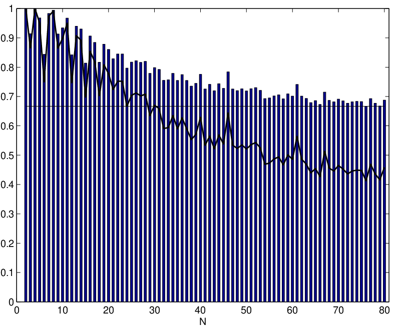
Fig.2, shows various interesting features of our protocol. The plot also shows that in addition to $N=2$, which is perfect (a well known fact for the Heisenberg interaction divincenzo), $N=4$ gives perfect ($F=1.000$) quantum state transfer to $3$ decimal places and $N=8$ gives near perfect ($F=0.994$). The fidelity also exceeds $0.9$ for $N=7,10,11,13$ and $14$. Till $N=21$ we observe that the fidelities are lower when $N$ is divisible by $3$ in comparison to the fidelities for $N+1$ and $N+2$. The plot also shows that a chain of $N$ as high as $80$ exceeds the highest fidelity for classical transmission of the state i.e., $2/3$ horodecki1 in the time interval probed by us. Of course the above results hold only when one is trying to directly transmit the quantum state over a distance. If one first shares entanglement through the channel, then the amount of entanglement $\cal{E}$ is about $0.45$ for an $80$ spin chain. This entanglement can be distilled to pure singlets and used for perfect teleportation.

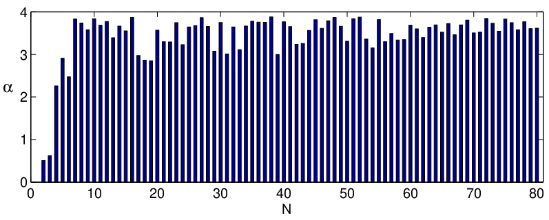
We will now like to estimate the entanglement sharable through chains so large that it is difficult to identify an optimal $t_{0}$ by numerical search. Hence we will choose $t_{0}$ according to a fixed (in general, non-optimal) prescription. To motivate this choice, we expand $e^{-iE_{m}t_{0}}$ in Eq.(10) as a Bessel function series to obtain

where $\beta_{0}=2Jt_{0}$. Using, $J_{N}(N+\xi N^{1/3})\approx(2/N)^{1/3}Ai(-2^{1/3}\xi)$ for large $N$ childs, (where $Ai(.)$ is the Airy function) we can prove that we get a maxima of $J_{N}(\beta_{0})$ at $t_{0}=(N+0.8089N^{1/3})/2J$ and at this time

which ranges from $0.135$ for $N=1000$ to $1.35\times 10^{-4}$ for $N=10^{12}$ (just $3$ orders decrease in ${\cal E}$ for an increase in length $N$ by $9$ orders – a very efficient way to distribute entanglement). Thus for any finite $N$, however large, the chain allows us to distribute entanglement of the order $N^{-1/3}$ in a time $t_{0}$ linear in $N$.

As an alternate system, we now consider a ring of $2N$ spins with Hamiltonian ${\bf H}_{\bf R}$ obtained by using $J_{ij}=(J/2)\delta_{i\oplus 1,j},B_{i}=B$ in Eq.(1)($\oplus$ is summation modulo $2N$). Alice and Bob access the spins at diametrically opposite sites ($s=1$, $r=N+1$). In this case, the $2N$ eigenstates in the one excitation sector are $|\tilde{m}\rangle_{\bf R}=(1/\sqrt{2N})\sum_{j=1}^{2N}e^{i\frac{\pi}{N}(m-1)j}|{\bf j}\rangle$ and

where $u_{m}=\exp(-iE_{m}t_{0})$ and $IDFT_{r-s}(u_{m})=(1/2N)\sum_{m=1}^{2N}u_{m}\exp\{i(2\pi/2N)(r-s)(m-1)\}$ is the $(r-s)$th component of the inverse discrete fourier transform of the vector $\{u_{m}\}$. Eqs.(11) and (13), and the nature of Bessel functions, imply that the maxima of ${\cal E}$ coincide for the line and the ring. This means that by using a ring you can communicate as efficiently over a distance $r-s=N$ as you can with a open ended line over a distance $r-s=N-1$. An immediate implication is that a $4$ spin ring allows perfect communication between diametrically opposite sites (because a $2$ spin line does divincenzo). This simple result in quantum information was not known till now. The coincidence of the maxima also means that the maxima of ${\cal E}$ for the line can also be computed by inverse fourier transforming $\{u_{m}\}$.

We now mention potential systems for realization. Josephson junction arrays, excitons in quantum dots and real 1D magnets, which motivated the recent study of quantum computation in Heisenberg chains zhou; benjamin will be good candidates. Interactions in such systems are difficult to tune. Our scheme can be implemented in such systems without the elaborate control required for quantum computation. 1D arrays of spins in solids divincenzo; kane are also candidates. There are ring molecules described exceptionally well by ${\bf H}_{\bf R}$, which also allow local probes for individual spins loss (these are antiferromagnetic, but a large $B$ could make $|{\bf 0}\rangle$ the ground, and $|\tilde{m}\rangle_{\bf R}$ the first excited states). Benzene molecules (with NMR probes possible) with $J_{ij}=\frac{\delta_{i\oplus 1,j}}{4}+\frac{\delta_{i\oplus 2,j}}{12\sqrt{3}}+\frac{\delta_{i\oplus 3,j}}{32}$, still have $|\tilde{m}\rangle_{\bf R}$ as eigenstates bowden. $F$ can thus be calculated by an IDFT to be $0.793$ for $r-s=3$ at $t_{0}=130$. Principles of the scheme should also be testable in simulated open ended Heisenberg chains in a 1D optical lattice duan.

In this letter, I have presented a protocol for quantum communication through an unmeasured and unmodulated spin chain. It allows quantum communication between adjacent quantum computers without interfacing different physical systems. It is well known that there exists an alternate trivial method of transferring quantum states perfectly over a distance by a series of swaps. But that requires an elaborate sequence of time dependent fields. The highly non-trivial finding of this letter is that even without doing anything, simply by placement, quantum states can be transmitted with high fidelity over a significant distance and entanglement of the order $N^{-1/3}$ can be shared across a chain of length $N$. We also found that a $4$ spin ring allows perfect quantum communication between diametrically opposite sites. This letter can be regarded as a study of a fundamental condensed matter system (a finite ferromagnet and its excitations) from the viewpoint of quantum communications. There remains an enormous scope for future extensions to spin graphs of varied geometry and interactions and to other well known condensed matter systems.

This work is supported by the NSF under Grant Number EIA-00860368. I thank G. J. Bowden, J. Eisert, A. Ekert, J. Harrington, V. Korepin, R. Raussendorf, A. Thapliyal, F. Verstraete and particularly Michael Nielsen and John Preskill, for remarks and suggestions.

References

- (1) C. H. Bennett and D. P. DiVincenzo, Nature 404, 247 (2000).
- (2) C. H. Bennett et. al., Phys. Rev. Lett. 70, 1895 (1993).
- (3) D. Kielpinski, C.R. Monroe, and D.J. Wineland, Nature 417, 709 (2002).
- (4) X. Zhou et. al., Phys. Rev. Lett. 89, 197903 (2002).
- (5) S. C. Benjamin and S. Bose, Phys. Rev. Lett.(2003).
- (6) W. K. Wootters, Phys. Rev. Lett. 80, 2245-2248 (1998).
- (7) M. Horodecki, P. Horodecki, and R. Horodecki, Phys. Rev. Lett. 78, 574-577 (1997).
- (8) J. Preskill, Physics 219: Quantum Computation, http://www.theory.caltech.edu/people/preskill/ph229/.
- (9) M. A. Nielsen and I. L. Chuang, Quantum Computation and Quantum Information, Cambridge University Press, 2000.
- (10) This generality was pointed out to me by M. A. Nielsen.
- (11) D. Loss and D. P. DiVincenzo, Phys. Rev. A 57, 120 (1998).
- (12) M. Horodecki, P. Horodecki, and R. Horodecki, Phys. Rev. A 60, 1888 (1999).
- (13) A. M. Childs et. al., quant-ph/0209131.
- (14) B. E. Kane, Nature, 393, 133 (1998).
- (15) F. Meier and D. Loss, Phys. Rev. Lett. 86, 5373 (2001).
- (16) G. J. Bowden, J. Math. Chem. 31, 363 (2002).
- (17) L.-M. Duan, E. Demler, M. D. Lukin, cond-mat/0210564.