Classical limit for the scattering of Dirac particles in a magnetic field.
Abstract
We present a relativistic quantum calculation at first order in perturbation theory of the differential cross section for a Dirac particle scattered by a solenoidal magnetic field. The resulting cross section is symmetric in the scattering angle as those obtained by Aharonov and Bohm (AB) in the string limit and by Landau and Lifshitz (LL) for the non relativistic case. We show that taking in our expression of the differential cross section it reduces to the one reported by AB, and if additionally we assume our result becomes the one obtained by LL. However, these limits are explicitly singular in as opposed to our initial result. We analyze the singular behavior in and show that the perturbative Planck’s limit () is consistent, contrarily to those of the AB and LL expressions. We also discuss the scattering in a uniform and constant magnetic field, which resembles some features of QCD.
pacs
3.65.Nk, 11.15.Bt, 11.80.-m, 11.80.Fv1 Introduction.
We know that in the classical scattering of charged particles by magnetic fields the scattered particles describe circular trajectories with fixed radii, so they have a preferential direction of motion. In this work, the relativistic quantum version of the problem is studied in the lowest order of perturbation theory and a symmetric behavior in the scattering angle is found for uniform and solenoidal magnetic fields. We focus on the study of some interesting limit cases of the differential cross section and compare them with previous non relativistic results reported by Aharonov and Bohm (AB) [1] and Landau and Lifshitz (LL) [2].
Although the scattering of charged particles by a solenoidal magnetic field, Aharonov-Bohm (AB) effect has been studied perturbatively before by other authors [3], in this work we are interested in the classical limit of the differential cross section.
As it is known, the AB effect [1] is considered one of the most important confirmed [4] predictions of the quantum mechanics because it shows that the vector potential has a physical significance and can be viewed more than a mathemathical convenience. The interest in this effect has been increased recently. Both because of basic reasons that have changed the understanding of gauge fileds and forces in nature and also because it has a lot of connections with new physics, like the quantum Hall effect [5], mesoscopic physics [6] and physics of anyons [7].
In the last two decades, several treatments to the AB scattering problem have appeared. First, the magnetic phase factor in the non relativistic case was treated directly (e.g. [8]). Works that consider spin have also been carried out and specially the behavior of the wave function is studied taking into account a delta function like potential at the origin [9]. Although originally AB solved the problem exactly, the perturbative analysis has played an important role [10, 11, 3], giving rise to discussions about the form in which the incident wave must be treated [12]. Also, various QED processes of scalar and Dirac particles in the AB potential have been carried out, and special interest has been devoted to polarization properties in bremsstrahlung and synchrotron radiation [13, 14].
Our interest in this problem stems from the fact that an electron in a uniform infinite magnetic field is trapped in two dimensions in a potential of the harmonic oscillator form. Thus it is a confined point-like fermion and therefore resembles the dynamic confinement produced in Quantum Chromodynamics (QCD) for quarks in three dimensions. In order to keep our analogy as close as possible to the parton model ideas our computation is done in a perturbative fashion. In this model, the use of free particle asymptotic states is very common, nevertheless with a simple model calculation in Quantum Electrodynamics (QED) we show that this procedure could be misleading at least in lowest order.
In this work we focus our analysis in the classical limit. First we are puzzled by the symmetric results of the differential cross section with respect to the scattering angle , in contradistinction to the classical scattering which favor an asymmetrical result. Second, the classical limit of field theory is a long unsolved problem, it is therefore tempting to understand the above mentioned quantum (symmetric) vs classical (asymmetric) results in order to clarify the classical limit: Are we in the presence of a process which is purely quantum in nature as LL suggest?
2 Previous results in the non relativistic case.
Let us recall two landmark results of the non relativistic case for the differential cross section of the scattering of electrons by solenoidal magnetic fields. Chronologically, the first result was presented by Aharonov and Bohm [1]. They obtain the exact solution for the scattering problem when the radius of the solenoid is very small for a constant magnetic flux, in fact they consider only a quanta of magnetic flux ( gauss cm2). Their result is11 1 In the paper of Aharonov and Bohm the cross section appears to be inversely proportional to , but the reference frame they use is such that is traslated by . Also the factor is not explicitly shown due to a change of variable ().:
| (1) |
Independently, Landau and Lifshitz [2] study the same scattering problem with the use of the eikonal approximation. Including only the contribution of the vector potential from the exterior of the solenoid, they obtain precisely the same as Aharonov and Bohm. Notice that this cross section is symmetric in .
Landau and Lifshitz compute the differential cross section for small scattering angles in the case of a small magnetic flux, , where perturbation theory is applicable, then , and the resulting cross section develops a singular behavior in :
| (2) |
They comment that the singular behavior of the cross section in when it goes to zero is specifically a quantum effect, without any further comment. We will study this problem in the next sections.
3 Solenoidal magnetic field in the relativistic case.
Let us consider the scattering of a Dirac particle by the magnetic field of a solenoid with a constant magnetic flux. This is a problem in which free particle asymptotic states can be used. The beam polarization will be taken into account. As mentioned before, this is a problem studied before by other authors also using perturbation theory, but here our interest is quite different. We want to study the classical limit of the result and discuss the proper way to get it.
Consider a long solenoid of lenght and radius centered in the axis. Inside of the solenoid, where , the magnetic field is uniform, , with being a constant, while outside the solenoid, where , the magnetic field is null. For , the magnetic flux will be constant: . We will follow the Bjorken and Drell convention [15].
A vector potential that describes such magnetic field for the interior of the solenoid is with . Outside the solenoid, the vector potential is , with . Using the Levi-Civita symbol in three indices, , the vector potential of the solenoid field can be written as
with the scalar potential . Replacing this vector potential in the matrix, equation (11), for Dirac particle solutions, equation (10), and , we obtain
Notice that there exists a global phase in the free particle wave function because the presence of a pure gauge field in the exterior of the solenoid, but it does not contribute to . For both integrals the parts that correspond to and are proportional to and , respectively. So the energy-momentum conservation in the scattering process is guaranteed and the particles do not change their momentum in the magnetic field direction. The integrals in the plane perpendicular to are
where and are the order Bessel functions [17]. In this form, the matrix for is:
We note that in the lowest order in the matrix there exists a net contribution from the interior of the solenoid, where the magnetic field is not null, in contradisctintion with the LL calculation, where only the vector potential of the exterior of the solenoid is considered.
Finally, the differential cross section per unit length of the solenoid is
Averaging over incident polarizations we obtain
and we note that this result does not depend on the final polarization. After some algebra we get
where . Finally, introducing and explicitly, we have
| (3) |
which has the same form whether or not the final polarization of the beam is actually measured ( or ). As can be observed, the differential cross section is symmetric in . This is reminiscent of the Stern-Gerlach result, in which an unpolarized beam interacting with an inhomogeneous magnetic field is equally split into two parts, each one with opposite spin. But, as we have mentioned before, equation (3) does not depend on the final polarization of the particles. Thus, this symmetric behavior of should be a consequence of the perturbation theory but notice that it is also present in non perturbative results like those of AB and LL.
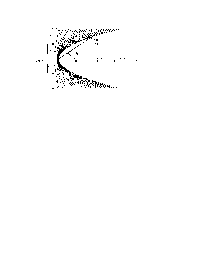
Figure 1 shows the behavior of the cross section of equation (3) in a polar plot scaled by a factor for a quanta of magnetic flux ( gauss cm2), cm and the energy of the incident particles running from 1 MeV to 50 MeV in steps of 2MeV as a function of the scattering angle .
When helicity states (HS) are considered, the resulting differential cross section is:
| (4) |
where and stand for the initial and final states of helicity and acquire only the values or . A zero differential cross section is obtained if . When , which implies helicity conservation, then the differential crosss section is:
| (5) |
which has the same form as equation (3).
4 Non-relativistic reduction.
To make connection with previous results, we study the limit case of small scattering angles. If we assume , then equation (3) (or equation (5)) reduces to
| (6) |
which agrees with the result reported by Aharonov-Bohm when . And if we impose in equation (6) the condition we obtain
| (7) |
which is presicely the result reported by Landau and Lifshitz.
We want to point out that it does not make sense to take the Planck’s limit () in equation (6) or in equation (7), because both expressions were obtained assuming the condition . Hence, we have to take the classical limit using the exprression for the differential cross section given in equations. (3) or (5).
5 Classical limit (Planck’s limit).
Let us study now the classical limit of the differential cross section of equation (3). For this purpose, consider the new adimensional variable and define . Observe that the limit implies or [16] for fixed . We can rewrite equation (3) as follows:
Because the asymptotic behavior of the Bessel function [17] is:
the resulting Planck’s limit of equation (3) is identically zero for fixed and :
| (8) |
which is also obtained for .
So, the perturbative result gives a consistent finite classical limit and reduces to the eikonal and the zero radius limits. If the classical limit is attempted in equations. (6) or (7), the result would be singular in , but this is clearly a misleading procedure.
The apparent difference in the classical limits of equation (3) (see equation (8)) and equations. (6) and (7) comes from the fact that in taking the limit of the perturbative result, equation (3), the Bessel function decreses as and it does generate an contribution to the cross section. On the other hand, if one begins by taking , the Bessel function approximates to , and this behaves like . The overall difference between these two procedures is an factor. It is important to notice that loop corrections to the perturbative expansion do not modify the behavior of the amplitude, this can be proved with the use of the loop expansion.
6 Quantized magnetic flux.
One can obtain a non divergent expression for the Landau-Lifshitz and the Aharonov-Bohm results when if in place of one fixes , the magnetic flux. The rationale behind this is that instead of a classical limit, with fixed , one imposes the magnetic flux quantization condition, .
For a quantized magnetic flux, where gauss cm2, the cross section of equation (3) takes the form
which apart of being independent of the charge of the particles, is a cross section of a purely quantum effect. Cast in this way it is not singular in as in the form that Landau-Lifshitz report. In particular, for the case of small scattering angles, it takes the form
| (9) |
which also has a null classical limit. If we recall equation (2) obtained by Landau-Lifshitz, we see that the same form can be recovered when , but these authors did not quantize the magnetic flux and thus they cannot get a cross section of a pure quantum problem as that of equation (9).
Also note that the zero classical limit with quantized magnetic flux of equation (1) is obtained:
7 Conclusions.
In this work we present a relativistic quantum study in first order of perturbation theory of the cross section of the scattering of a Dirac particle with magnetic fields. We have specially focused in the classical limit for the solenoidal magnetic field case.
In order to fulfill the perturbation theory requirements the magnetic field was bounded to a solenoidal one with constant flux. We obtained that the cross section of the scattering problem is given by equation (3) and has the same form whether or not the final polarization of the beam is actually measured. This indicates that the symmetry in the scattering angle is most likely a consequence of the perturbation theory.
We have shown that taking our result reduces to that one reported by Aharonov-Bohm. Also, our result agrees with that one obtained by Landau-Lifshitz when we take and . Notice that both cases lead to similar singular behavior in (see equations. (6) and (7)).
We have shown that the perturbative classical limit for all scattering angles and all radii of the solenoid with and fix, is identically zero, because the cross section behaves like and hence it is not singular in as the one of Landau-Lifshitz (see equation (2)). We point out that the same zero classical limit can be obtained in the limit with fixed and . Notice that the apparent difference in the classical limits comes from the fact that the asymptotic behavior of the Bessel function goes like and it does generate an contribution to the cross section, while taking first the approximation , the Bessel function behaves like . So, the overall difference between these two procedures is an factor.
When the magnetic flux is quantized, the cross section is proportional to getting, again, a null classical limit. This limit can be recovered from the Aharonov-Bohm and Landau-Lifshitz results because and then
an independent result of .
Finally we want to point out that althought our reslut is consistent in the sense that the Aharonov-Bohm and the Landau-Lifshitz results are recovered, there is not a direct classical correspondence via the Planck’s limit (see equation (8)), because in particular the cross section is symmetric in . This problem is shared also by the AB and LL solutions and is possibly solved by higher order corrections in the external magnetic field.
Uniform and constant magnetic field in the relativistic case.
Here we consider the scattering of a Dirac particle by an external uniform and constant magnetic field with a constant, described by the vector potential
As in perturbative QCD we take initial and final states as asymptotic states of free particles with momentum and spin , explicitly:
| (10) |
At first order in perturbation theory the scattering matrix is given by
| (11) |
where and with the Dirac matrices. If the initial state has momentum in the direction, the matrix for is
where we have denoted and similarly for . The integrals can be solved immediately because three of them are proportional to a Dirac delta function, while the integral in the direction is equal to . Then, the matrix of this problem is
where is the momentum transfer.
With the usual replacement of , we obtain the differential cross section per unit of magnetic field volume:
| (12) |
Note that the resulting differential cross section is proportional to a Dirac delta function of the momentum transfer in the incident direction of the particles, meaning that the particles do not change their momentum after their interaction with the magnetic field. This is in apparent contradiction with the common sense, because we know that in the classical situation a particle that interacts with a magnetic field changes its momentum, and its orbit is a circumference. Also note that we assumed that the magnetic field fills all the space and we used free particle solutions to solve the scattering problem. These conditions are physically questionable because the presence of the magnetic field binds the particles and therefore the asymptotic sates cannot be plane waves, just like is done in perturbative QCD.
To use perturbation theory it is necessary to verify its applicability limits. For perturbation theory to be valid one must satisfy [18] where is significant in the range and is the mass of the particle. For the case we are studying the range of the potential is infinite, so to use perturbation theory we need to modify the potential in such a way that it goes rapidly to zero at infinity, doing the system compatible with our calculation and with physics, and then the particles can be treated as free asymptotically.
References
- [1] Aharonov A and Bohm D 1959 Phys. Rev. 115 485
- [2] Landau L D and Lifshitz E M 1977 Quantum Mechanics (non relativistic theory) (Oxford: Pergamon Press)
- [3] Boz M and Pak N K 2000 Phys. Rev. D 62 045022
- [4] Chambers R G 1960 Phys. Rev. Lett. 5 3 Osakabe N et al. 1986 Phys. Rev. A 34 815
- [5] Laughlin R B 1983 Phys. Rev. Lett. 50 1395 Halperin B I 1984 Phys. Rev. Lett. 52 1583 Giacconi P and Soldati R 2000 J. Phys. A 33 5193
- [6] Liu J et al. 1993 Phys. Rev. B 48 15148 de Vegvar P G N et al. 1989 Phys. Rev. B 40 3491 Timp G et al. 1989 Phys. Rev. B 39 6227
- [7] Ouvry S 1994 Phys. Rev. D 50 5296 Chou C, Hua L and Amelino-Camelia G 1992 Phys. Rev. Lett. B 286 329 and references there in Chou C 1991 Phys. Rev. D 44 2533 Comtet A, Mashkevuciha S and Ouvry S 1995 Phys. Rev. D 52 2594 Gomes M and da Silva A J 1998 Phys. Rev. D 57 3579 Lin Q 2000 J. Phys. A 33 5049
- [8] Berry M V 1980 Eur. J. Phys. 1 240
- [9] Hagen C R 1990 Phys. Rev. Lett. 64 503
- [10] Hagen C R 1995 Phys. Rev. D 52 2466
- [11] Gomes M, Malbouisson J M and da Silva A J 1997 Phys. Lett. A 236 373
- [12] Sakoda S and Omote M 1997 J. Math. Phys. 38 716
- [13] Audretsch J and Zkarzhinsky V D 1998 Found. Phys. 28 777
- [14] Bagrov V G, Gitman D M, and Tlyachev V B 2001 Nucl. Phys. B 605 425
- [15] Bjorken J D and Drell S D 1964 Relativistic Quantum Mechanics (New York: McGraw-Hill)
- [16] Zkarzhinsky V D and Audretsch J 1997 J. Phys. A 30 7603
- [17] Arfken G 1970 Mathematical Methods for Physicists (Oxford: Academic Press)
- [18] Joachain C J 1975 Quantum Collision Theory (Amsterdam: North-Holland)