[
Numerical study of induced vortex tunneling
Abstract
Tunneling of vortex-antivortex pairs across a superconducting film can be controlled via inductive coupling of the film to an external circuit. We study this process numerically in a toroidal film (periodic boundary conditions in both directions) by using the dual description of vortices, in which they are represented by a fundamental quantum field. We compare the results to those obtained in the instanton approach.
pacs
PACS numbers: 85.25.Hv, 03.67.Lx]
I Introduction
Persistent-current superconducting devices, in which the basis states are characterized by different values of the enclosed flux, are interesting physical systems in their own right and are also promising candidates for applications to quantum memory. The possibility to form quantum superpositions of macroscopic flux states has been demonstrated in experiments with SQUIDs [1, 2].
Once reliable storage of quantum superpositions is achieved, it becomes necessary to consider possible mechanisms for reading and writing operations and for assembling several such individual units (qubits) into a scalable quantum computer. In SQUIDs, various proposals have exploited the existence of a potential barrier between two stable basis states and have involved manipulation of the barrier itself, use of tunneling effects, or a controlled excitation over the barrier [3, 4].
In this paper, we examine a model which describes tunneling of vortices (short Abrikosov flux lines) in a ring of thin superconducting film. We consider a scheme in which a pulse of supercurrent suppresses superconductivity, thus lowering the potential barrier and inducing tunneling, see Fig. 1. Because this process changes the flux enclosed by the ring, it can be used to form arbitrary superpositions of the basis states. We will see that in a suitable geometry, it is possible also to independently control the energy bias between the basis states, similarly to how it is done in SQUIDs. On the other hand, this device does not contain any Josephson junctions, thereby avoiding dissipation due to various fabrication issues, such as defects in the insulating barrier.
Motivated by these observations, we consider a simplified model, convenient for numerical work, in which the film has periodic boundary conditions in both directions, forming a torus. The suppression of superconductivity and the biasing flux are represented in this model by two independent parameters: the vortex pair-production frequency , and the driving force .
For applications to quantum computing, of main interest is the adiabatic regime, when there is very little residual excitation left in the system after the pulse (in other words, no real, as opposed to virtual, vortex pairs are produced). If this condition were not satisfied, the remaining vortices would be easily “detected” by the environment (e.g. by electrons at the vortex cores), and that would result in rapid decoherence. Thus, we envision a situation when a virtual vortex and an antivortex are created, say, on the inside of the torus, transported along the opposite semicircles to the outside, and annihilated there, almost without a trace.

In thin films, the elastic mean-free time of electrons is short [5]; for a film of thickness we use . This results in a strong suppression of the Magnus force on the vortex and a relatively small friction [6, 7, 8, 9]. In addition, and in contrast to motion of real vortices, the density of normal electrons at the vortex core during tunneling is a variational parameter, which adjusts itself to maximize the tunneling rate. This leads to further cancellation of the Magnus force and a reduction in the inertial mass of the vortex.
There are two theoretical approaches to induced vortex transport. One is based on instantons, solutions to the Euclidean equations of motion. Using the expressions [6, 8] for the friction caused by the core fermions, we find that it results in the following contribution to the Euclidean action:
| (1) |
where is the electron density, is the width of the film, and . Using Å-1, , m, and nm, we obtain . By itself, this is not a small number, but the crucial point is that depends quadratically on the gap . So, when we suppress by a pulse of current, we also reduce . In fact, the dependence of on is precisely the same as that of the vortex pair-production frequency . So, in what follows we simply include the effect of the friction in our definition of .
The driving force , due to the energy bias between the basis states, can be viewed as a Lorentz force caused by an effective electric field, , in the direction. Then, the average vortex current due to tunneling is obtained in the instanton approach as [10]
| (2) | |||||
, and the magnitude of the electron charge. In (2), the first term is due to instantons, and the second to anti-instantons; is the real part of the instanton action, and is the limiting speed of vortex motion.
The second method is entirely real-time. Vortices are described by a fundamental quantum field, and a nonzero average vortex current comes out as a result of the discreteness of field modes. The periodicity in has been confirmed analytically in this approach [10], provided the vortex-antivortex potential can be replaced by its average and included as an additional contribution to . The second principal effect seen in (2)—the dependence—has been confirmed only for the case of small , . It is of interest to develop this approach further, so that it can be applied also to cases with large and a non-trivial potential. The present paper addresses, via numerical integrations, the first part of this program.
In practice, it may be easier to fabricate a thin strip than a thin cylinder. The field-theoretical method will apply to that case as well, provided one can establish the boundary conditions for the vortex field at the edges of the strip.
The paper is organized as follows. In Sect. II we discuss how one can independently control the vortex mass and the driving force in a thin superconducting ring. In Sect. III, we discuss the real-time description of vortex tunneling. Numerical results are presented in Sect. IV, and a summary in the concluding Sect. V.
II Control of current and flux in thin superconductors
Consider a uniform superconducting ring inductively coupled to an external circuit. Suppose the order parameter winds times around the ring. Then, the London current can be expressed through the flux enclosed by the ring as
| (3) |
Here is the flux quantum, and is the “kinetic” inductance:
| (4) |
is the density of superconducting electrons, is the cross-sectional area, and is the length of the ring.
We have introduced the London penetration depth , and because superconductivity can be deliberately suppressed by some means, is in general different from the unperturbed penetration depth . Recall also that in a thin film determines the strength of the London current, but not the screening length of the magnetic field [11].
The flux in (3) is the total flux, which consists of the flux created by the external circuit and that created by the current itself:
| (5) |
where is the ordinary inductance of the ring. Using this together with eq. (3), we can express the supercurrent through :
| (6) |
Even though and enter eq. (6) symmetrically, there is an essential difference between them, since depends only on the geometry and in this sense is a constant, while depends on .
So, there are two distinct limits of eq. (6). If , i.e., the cross-sectional area is large enough, then according to (6) controls the current. On the other hand, if , determines only the product , i.e., the ratio .
In the second, thin-ring, regime, by a slow variation of we can smoothly change the order parameter from a large initial value, for which vortex tunneling will be strongly suppressed, to some much smaller values that allow tunneling, and then back to the initial state. For small, slowly changing , this can be seen directly from the Ginzburg-Landau (GL) equation:
| (7) |
where is the current density, is a critical velocity ( is the coherence length), and , are GL parameters. If quantum coherence can be preserved during this process, such a device would be reliable quantum memory.
Now, , so the crossover between the thick and thin-ring cases occurs at
| (8) |
Assuming that the logarithm is of order unity, and using an unperturbed value nm, we obtain
| (9) |
When (which is proportional to ) is suppressed to allow tunneling, and, consequently, grow, so if the condition held in the initial state, it would hold even better during tunneling.
According to this estimate, if the ring is made from a thin film, it does not have to be particularly narrow to achieve the thin-ring condition . For example, for thickness nm, the estimate (9) allows for widths as large as m.
As a specific example of how can be suppressed by a pulse of current, consider the double-arm geometry shown in Fig. 1. It is convenient to imagine that the wire carrying the constant current is closed at a large distance, so that the device can be viewed as a superposition of two closed circuits, with currents and . In addition to kinetic inductances , , the circuits have self-inductances , and a mutual inductance . We can also define and . Consider regime when the inductance of arm 1 is mostly kinetic, , while that of arm 2 is mostly ordinary, . Then, the currents in the arms are
| (10) | |||||
| (11) |
where . Suppose further that . In this case, we see from (10) that the current controls the parameter , which according to (7) determines how close the first arm is to criticality.
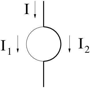
The inductive energy of the double-arm device is
| (12) |
where is independent of and the external flux. If the device is biased by half a flux quantum, , the energy (12) has two degenerate minima at . If deviates from half-quantum by a small amount , the energy difference between the two minima is . This results in an additional force
| (13) |
acting on a vortex as it tunnels across arm 1. Note that unlike the case of a single current-biased superconducting wire [12], this force is not related to the total current but is an independently controlled parameter. The only restriction is that should not exceed the energy of vortex pair production, so that no real vortices are able to nucleate.
III Real-time description of vortex tunneling
Motivated by the arguments of the preceding sections we consider a model of vortex tunneling, in which the main force acting on the vortex is the driving force (13). The requisite suppression of the order parameter is achieved by some independent means, such as a pulse of external current in the double-arm device.
In the real-time approach, vortices are described by a quantum field [13], which in our case obeys the equation of motion
| (14) | |||||
| (15) |
Here is the thickness of the film, is the magnitude of the electron charge, and is a time dependent electric field produced by the changes in and . The speed is the limiting speed of vortex motion: in the second-quantized description (15) it plays the role analogous to the speed of light in relativistic quantum theory.
The driving force is represented by the potential
| (16) |
Such an explicit -dependence in the equation is inconvenient for numerical work. However, it is possible to make a transformation of the field , similar to a gauge transformation, so that the force disappears from the first term in (15) and appears instead as an addition to the electric field :
| (17) | |||||
| (18) | |||||
| (19) |
In what follows, we will use the same notation for the transformed field as we used for the original one.
In general, the transformations (17)–(19) lead to one spurious effect. Imagine that starts from zero at , goes through nonzero values near and then back to zero at . Then, according to eq. (15), has no effect at , while according to (19) the correction to is still nonzero (and proportional to the integral of ). Fortunately, owing to the periodic dependence of vortex transport on , cf. eq. (2), this correction is immaterial provided satisfies a quantization condition:
| (20) |
where is an integer. Only in this case the problem obtained by the transformations (17)–(19) is equivalent to the original problem (15).
The transformed equation has no explicit dependence on and can be solved by the mode expansion
| (21) |
where , and are annihilation operators for vortices and antivortices, respectively, and are the mode functions that take into account the time dependence of and of the vortex “mass” . We have assumed that the vortex field has periodic boundary conditions in both directions.
Substituting the expansion (21) into the field equation, we obtain the equation for the mode functions:
| (22) |
where
| (23) |
and . We consider the case of effectively zero temperature, when there are no vortices in the initial state. So, eq. (22) is solved with the vacuum initial conditions
| (24) |
where is the two dimensional volume of the film, is some initial moment of time, , and .
Once a solution to the initial problem (22)–(24) is available (e.g., from a numerical integration), one can obtain various quantities of interest as averages over the vacuum of the operators and . In what follows, we consider three such quantities: the average vortex current, the energy, and the vortex occupation numbers, all as functions of time.
Only the component of the average vortex current is nontrivial. It can be found by averaging the operator expression
| (25) |
over the vacuum of and , to obtain
| (26) |
where
| (27) |
If we integrate (26) over time, we will obtain the average vortex number transported in the direction per unit length in the direction during the entire pulse. This is a convenient measure of vortex transport.
At zero temperature, and for a sufficiently adiabatic pulse, the only source of vortex transport is vortex tunneling. In the real-time formalism, the corresponding contribution to the current (26) appears as a result of the discreteness of modes. It is exponentially suppressed with and should reproduce the result (2) of the instanton approach.
We should be careful, however, about the ultraviolet regularization of eq. (27). A sharp momentum cutoff is not adequate for our purposes, especially since we need a regulator that would preserve the symmetry under the transformation (17)–(19). A suitable choice is a Pauli-Villars regulator—an additional field with a very large “mass” , whose contribution is added to (26) with an opposite sign relative to that of . If the maximal is some , the regulator contribution to (27) can be computed analytically. Both the pair production and tunneling are negligible for large , so we replace the regulator mode functions with their WKB expressions, and the sum over with an integral, to obtain
| (28) |
The resulting expression for at finite (large) value of is then
| (29) |
and the full regularized expression is
| (30) |
IV Numerical Results
As discussed in Sect. II, it is possible to consider geometries in which the suppression of the order parameter and the driving force on the vortex are entirely independent functions of time. For example, in the double-arm geometry of Fig. 2, the suppression is determined by the externally controlled current , while the driving force, by the biasing flux. Accordingly, we consider here a situation when the order parameter is suppressed for a relatively long time down to some value that allows tunneling, while the driving force exists only for a shorter time: its biases tunneling and leads to a nonzero value of the average (26).
A convenient parametrization of the force is obtained by defining an effective current related to by an effective Maxwell equation
| (31) |
For a sufficiently adiabatic pulse, the first term here is much smaller than the second, and we neglect it in what follows. According to eq. (7), it is , i.e., a quantity akin to the vector potential, that determines how close the film is to criticality. So, we define an effective vector potential via the London formula
| (32) |
Combining (31) (with ) and (32), we obtain
| (33) |
where is the fine-structure constant, and is the critical vector potential.
We consider only biasing pulses that have very small ratios. Such pulses do not significantly modify . So, the only difference between and the unperturbed value of the penetration depth is due to the broader pulse of the current . Similarly, the vortex “mass” during the biasing pulse may be assumed constant and equal to some .
For the parameters of the film, we take nm, nm, and nm. The latter two values take into account the suppression of and the increase in due to the small value of the thickness [14]. The sizes of the film are m and m.
We assume that the suppression of superconductivity by a pulse of has reduced by a factor of 25. Then, . In our numerical integrations, we keep and the form of the pulse fixed and scan over different values of .
The limiting vortex speed can be obtained by estimating the inertial mass of the vortex and taking the ratio . In many cases, the main contribution to comes from the small variation of electron density at the vortex core. In this case, , and [15, 16, 17]. However, when we search for an optimal tunneling path in the Euclidean time, the density at the core becomes a variational parameter, and it is advantageous for it to differ from the average density as little as possible. In this case, the main contribution to comes from the electric field produced by the moving vortex, resulting in a much larger [15]. For the above values of the parameters, we use .
In what follows, we adopt the system of units in which and all lengths are measured in microns. Thus, the unit of time is ps.
The easiest way to implement the quantization condition (20) is to consider whose integral over time is zero. We set
| (34) |
and take and . The latter corresponds to 2 ps.
Equation (22), with
| (35) |
and different values of was integrated numerically using a Runge-Kutta sixth-order integrator. We use values of : , with .
Taking the limit in eq. (30) requires correcting the numerical data at least by terms of order . In our case, . The correction was computed by assuming that it dominates the transport already for , which is a large enough value to significantly suppress tunneling.
In Fig. 3 we plot the total vortex transport
| (36) |
for and several values of ; . The data are well fit by a curve proportional to , which is the instanton exponential. Note that in this calculation the maximal value of is , which exceeds the mode spacing . For , agreement between the instanton and real-time calculations was confirmed analytically in ref. [10]. We now confirm the agreement beyond the small limit.

Because for all values of in Fig. 3, the transport is to a good accuracy adiabatic. The measure of adiabaticity is the vortex occupation numbers
| (37) |
where
| (38) |
are the energies (divided by ) of the individual modes. In Fig. 4 we plot the total occupation number
| (39) |
for and . We see that there is practically no residual excitation (real vortex-antivortex pairs) in the final state: at , we obtain .

V Conclusion
The results of this work are two-fold. First, we have shown that in certain geometries (such as the double-arm geometry of Sect. II), it is possible to independently control the driving force acting on a vortex as it tunnels across a superconducting film and the suppression of superconductivity in the film (i.e., the mass of the vortex). Motivated by this observation, we have then considered a model problem of vortex tunneling in a toroidal film. The driving force is modeled by an effective electric field, which biases tunneling and results in a nonzero average vortex current.
Second, we have used this model setup to study the dependence of the tunneling rate on the vortex “mass” (more precisely, the pair-production frequency) in the real-time approach, in which vortices are represented by a fundamental quantum field. We have confirmed the exponential dependence on the “mass” found in the instanton (Euclidean) approach. We have also confirmed that a sufficiently slow, adiabatic variation of the biasing field can lead to a sizeable vortex current without any real vortex-antivortex pairs remaining in the final state. This means that induced vortex transport may be a suitable technique for applications requiring a high-degree of quantum coherence, such as quantum memory.
References
- [1] J. R. Friedman et al., Nature, 406, 43 (2000).
- [2] C. H. van der Wal et al., Science, 290, 773 (2000).
- [3] X. Zhou et al., IEEE Trans. Appl. Supercond. 11, 1018 (2001) [quant-ph/0102090].
- [4] M. Crogan, S. Khlebnikov, and G. Sadiek, Supercond. Sci. Technol. 15, 8 (2002) [quant-ph/0105038].
- [5] K. Fuchs, Proc. Cambridge Phil. Soc. 34, 100 (1938).
- [6] N. B. Kopnin and V. E. Kravtsov, Pis’ma ZhETF 23, 631 (1976) [JETP Lett. 23, 578 (1976)].
- [7] G. E. Volovik, Zh. Eksp. Teor. Fiz. 104, 3070 (1993) [JETP 77, 435 (1993)].
- [8] A. van Otterlo, M. Feigel’man, V. Geshkenbein, and G. Blatter, Phys. Rev. Lett. 75, 3736 (1995).
- [9] M. V. Feigel’man, V. B. Geshkenbein, A. I. Larkin, and V. M. Vinokur, Pis’ma ZhETF 62, 811 (1995) [JETP Lett. 62, 834 (1995)].
- [10] S. Khlebnikov, quant-ph/0210019.
- [11] J. Pearl, Appl. Phys. Lett. 5, 65 (1964).
- [12] L. I. Glazman and N. Ya. Fogel, Fiz. Nizk. Temp. 10, 95 (1984) [Sov. J. Low Temp. Phys. 10, 51 (1984)].
- [13] P. Ao, J. Low Temp. Phys. 89, 543 (1992).
- [14] M. Tinkham, Phys. Rev. 110, 26 (1958).
- [15] H. Suhl, Phys. Rev. Lett. 14, 226 (1965).
- [16] M. Yu. Kupriyanov and K. K. Likharev, ZhETF 68. 1506 (1975) [Sov. Phys. JETP 41, 755 (1975)].
- [17] G. Blatter, V. B. Geshkenbein, and V. M. Vinokur, Phys. Rev. Lett. 66, 3297 (1991).