The Casimir force and the quantum theory of lossy optical cavitiesUnité de l’Ecole Normale Supérieure, de l’Université Pierre et Marie Curie, et du Centre National de la Recherche Scientifique
Abstract
We present a new derivation of the Casimir force between two parallel plane mirrors at zero temperature. The two mirrors and the cavity they enclose are treated as quantum optical networks. They are in general lossy and characterized by frequency dependent reflection amplitudes. The additional fluctuations accompanying losses are deduced from expressions of the optical theorem. A general proof is given for the theorem relating the spectral density inside the cavity to the reflection amplitudes seen by the inner fields. This density determines the vacuum radiation pressure and, therefore, the Casimir force. The force is obtained as an integral over the real frequencies, including the contribution of evanescent waves besides that of ordinary waves, and, then, as an integral over imaginary frequencies. The demonstration relies only on general properties obeyed by real mirrors which also enforce general constraints for the variation of the Casimir force.
I Introduction
An important prediction of quantum theory is the existence of irreducible fluctuations of electromagnetic fields in vacuum. Besides their numerous observable consequences in microscopic physics, vacuum fluctuations also have observable effects in macroscopic physics, for example the Casimir force they exert on mirrors Casimir48.
Casimir calculated this force in a geometrical configuration where two plane mirrors are placed a distance apart and parallel to each other, the area of the mirrors being much larger than the squared distance . He considered the ideal case of perfectly reflecting mirrors and obtained an expression which, remarkably, depends only on the geometrical quantities and and on the fundamental constants and
| (1) |
This attractive force has been observed in a number of ‘historical’ experiments Deriagin57; Spaarnay58; Tabor68; Black68; Sabisky73 which confirmed its existence and main properties Sparnaay89; Milonni94; Mostepanenko97. Several recent experiments reached an accuracy in the % range by measuring the force between a plane and a sphere Lamoreaux97; Mohideen98; Roy99; Harris00 or two cylinders Ederth00. Similar experiments were also performed with MEMS Chan01s; Chan01p (see also Buks01). An experiment studied the plane-plane configuration considered by Casimir Bressi02 but, as a consequence of the difficulties associated with this geometry, reached only a 15% accuracy (see reviews of recent experiments in Bordag01; Lambrecht02).
The Casimir force is the most accessible experimental consequence of vacuum fluctuations in the macroscopic world while vacuum energy is known to raise a serious problem with respect to gravity and cosmology (see references in Reynaud01; Genet02). This is a reason for testing the predictions of Quantum Field Theory concerning the Casimir effect with the greatest care and accuracy. The theory of the Casimir force is also a key point for the experiments searching for the new weak forces predicted by theoretical unification models to arise at distances between nanometer and millimeter Carugno97; Fischbach98; Bordag99; Fischbach99; Long99; Hoyle01; Adelberger02; Long02. The Casimir force is indeed the dominant effect between two neutral objects at m or subm distances so that an accurate knowledge of its theoretical expectation is as crucial as the precision of measurements in such experiments Lambrecht00.
In this context, it is essential to account for the differences between the ideal case considered by Casimir and the real experimental situation. Recent experiments use metallic mirrors which show perfect reflection only at frequencies below their plasma frequency. They are performed at room temperature, with the effect of thermal fluctuations superimposed to that of vacuum fluctuations. In the most accurate experiments, the force is measured between a plane and a sphere, and not between two parallel planes. The surface state of the plates, in particular their roughness, should also affect the force. A large number of works have been devoted to the study of these effects and we refer the reader to Bordag01; Lambrecht02 for a bibliography.
The evaluation of the Casimir force between imperfect lossy mirrors at non zero temperature has given rise to a burst of controversial results Bostrom00; Svetovoy00; Bordag00; Lamoreaux01c; Sernelius01r; Sernelius01c; Bordag01r; Klimchitskaya01; Bezerra02; Lamoreaux02 which constitutes a part of the motivations for the present work. For the sake of comparing experimental measurements and theoretical expectations, it is necessary to have at one’s disposal a reliable expression of the Casimir force in the experimental situation. In the present paper, we focus our attention on the effect of imperfect reflection of the mirrors. Other effects, in particular the effect of temperature, will be addressed in follow-on papers.
We consider the original Casimir geometry with two perfectly plane and parallel mirrors. Except for these assumptions, we consider arbitrary frequency dependences for the mirrors which, in particular, may be lossy. We evaluate the Casimir force as the effect of vacuum radiation pressure on the Fabry-Perot cavity formed by the two mirrors. The net force results from the balance between the repulsive and attractive contributions associated respectively with resonant or antiresonant frequencies. It is obtained as an integral over the axis of real frequencies, including the contribution of evanescent waves besides that of ordinary waves. It is then transformed into an integral over imaginary frequencies by using physical properties fulfilled by all real mirrors.
The formula obtained here for the Casimir force turns out to be identical to the expression already published in Jaekel91 but the new derivation has a wider scope of validity than the previous one since it remains valid for lossy mirrors. The fact that the formula keeps the same form despite the widening of the assumptions is intimately related to a theorem which relates the spectral density of the fields inside the cavity to the reflection amplitudes seen by the same fields. This theorem was demonstrated in Jaekel91 and Barnett98 in specific cases and we prove it in the present paper without any restriction. To this aim, we introduce a systematic treatment of lossy mirrors and cavities as dissipative networks Meixner. We define scattering and transfer matrices for elementary networks like the interface between two media or the propagation over a given length in a medium. We then deduce the matrices associated with composed networks, like the optical slab or the multilayer mirror.
The results obtained in this manner are therefore applicable to a large variety of mirrors, still with the assumption of perfect plane geometry. In the particular case of a slab with a large width, the Lifshitz expression Lifshitz56; LLcasimir is recovered. At the limit of perfectly reflectors, the ideal Casimir formula (1) is obtained. More generally, the expression gives the Casimir force as an integral written in terms of the reflection amplitudes characterizing the two mirrors. This integral is finite as soon as the amplitudes obey the general properties of scattering theory already alluded to. In other words, the difficulties usually associated with the infiniteness of vacuum energy are solved by using the properties of real mirrors themselves rather than through an additional formal regularization technique.
We finally show that the same physical properties constrain the variation of the Casimir force. In particular, they invalidate proposals which has been done for ‘tayloring’ the force at will by using mirrors with specially designed scattering amplitudes Iacopini93; Ford93. In these proposals, the balance between attractive and repulsive contributions to the force is change, leading to the hope that the Casimir force could reach large or have its sign changed from an attractive force to a repulsive one Iacopini93. Using the simple model of a one-dimensional space, it has already been shown Lambrecht97 that these hopes cannot be met for arbitrary mirrors built up with dielectric layers. Here, the argument is generalized to the Casimir geometry in three-dimensional space with the following conclusions : the Casimir force cannot exceed the value obtained for perfect mirrors, it remains attractive for any cavity length and its value is a decreasing function of the cavity length. This is true for any mirror obtained by piling up layers of media described by dielectric functions. This definition of multilayer dielectric mirrors includes the case of metallic layers, provided that magnetic effects play a negligible role in the optical response.
II Vacuum field modes
As explained in the Introduction, we consider in this paper the original Casimir geometry with perfectly plane and parallel mirrors aligned along the directions and . This configuration obeys a symmetry with respect to time translation as well as transverse space translations along these directions. We use bold letters for two-dimensional vectors along these directions and denote the transverse position. As a consequence of this symmetry, the frequency , the transverse vector and the polarization are preserved throughout the scattering processes on a mirror or a cavity. The scattering couples only the free vacuum modes which have the same values for the preserved quantum numbers and differ by the sign of the longitudinal component of the wavevector.
In the present section, we introduce notations for the vacuum field modes, first in empty space and then in a dielectric medium. These notations are chosen to be well-adapted to the symmetry of the problem.
II.1 Vacuum modes in empty space
In empty space, the components of the wavevector are given for each field mode by the frequency , the incidence angle and the azimuthal angle
| (2) |
is the modulus of the transverse wavevector and the longitudinal component may be expressed in terms of the preserved quantities and
| (3) |
is defined as the sign of and represents the direction of propagation with and corresponding respectively to rightward and leftward propagation.
The two polarizations are defined by the transversality with the incidence plane of electric and magnetic fields respectively. They are given by the unit electric vectors
| (4) |
or, equivalently, the unit magnetic vectors and . For each mode, the wavevector and polarization vectors form an orthogonal spatial basis. We have chosen linear polarizations described by real components; hence the unit vectors and are not affected by the complex conjugation appearing below in the relation between positive and negative frequencies.
The two modes corresponding to the same values of , and but opposite values of are coupled by scattering on a mirror. For this reason, we introduce a label gathering the values of , and . A mode freely propagating in vacuum is thus labeled by and and the summation over modes is described by the symbols
| (5) | |||||
Note that appears implicitly as the sign of in the first form whereas it appears explicitly in the second one.
The free vacuum fields are then written as linear superpositions of modes
| (6) |
The vacuum impedance describes the electromagnetic constants in vacuum. In the following, the symbol will be reserved to the relative permittivity with the value 1 in vacuum.
The quantum field amplitudes and correspond to positive and negative frequency components. They fit the definition of annihilation and creation operators of quantum field theory and obey the canonical commutation relations CCT87
| (7) |
In the vacuum state, the anticommutators of quantum amplitudes are derived from the corresponding commutators
| (8) |
The dot symbol represents a symmetrized product.
II.2 Stress tensor in empty space
The energy density per unit volume is a quadratic form of the fields and
| (9) |
When subsituting the expression of free fields, is obtained as a bilinear form of the field amplitudes. Here, we study the averaged radiation pressure in the vacuum state which leads to a contraction in the sums over modes. Using the vacuum property (8), we find the averaged energy density in vacuum equal to the sum over the modes of
| (10) |
As it is well-known, this energy density is infinite.
The radiation pressure on plane mirrors oriented along directions is determined by the component of the Maxwell stress tensor
| (11) |
Here, the dot symbol represents a symmetrized product of the quantum amplitudes and, simultaneously, a scalar product of the vectors; the overline symbol describes the mathematical reflexion of a vector with respect to the plane
| (12) |
As for , averaging in vacuum state leads to a contraction over the modes with the result
| (13) | |||||
This expression is similar to the expression (10) of the energy density with an extra factor well-known in studies of radiation pressure. The sum over modes is still infinite but this infiniteness problem will be solved in the forthcoming calculation of the Casimir force.
II.3 Fields in dielectric media
In the following, we consider mirrors built up as dielectric multilayers. Each dielectric medium is characterized by a relative permittivity or, equivalently, an index of refraction depending on frequency. The magnetic permeability is kept equal to its vacuum value since this corresponds to all experimental situations studied so far. We stress again that this definition of dielectric mirrors includes the case of metals as long as the magnetic response plays a negligible role. We consider layers thick enough so that the dielectric response is local, i.e. described by a wavevector-independent permittivity .
We will sometimes take the plasma model as a first description of metallic optical response
| (14) |
where and represent respectively the plasma frequency and the plasma wavelength. This simple model is not sufficient for an accurate evaluation of the Casimir force between real mirrors Lambrecht00. To this aim, it is necessary to describe the optical response of metals with a dissipative part associated with electronic relaxation processes. As a consequence of causality, the real and imaginary parts of are related to each other through the Kramers-Kronig dispersion relations LLcausality.
For any function of frequency more generally, causality is unambiguously characterized in terms of analyticity properties : or are analytical functions of in the ‘physical domain’ of the complex frequency plane, that is the domain of frequencies with a positive imaginary part . This property is obeyed by other response functions to be encountered below and it will play an important role in the derivation of the Casimir force. We will introduce an equivalent notation for complex frequencies with the physical domain now defined by a positive real part for
| (15) |
The dispersion relation (2) is changed inside a refractive medium to
| (16) |
The preservation of and at the traversal of an interface is equivalent to the Snell-Descartes law of refraction.
The sign has to be carefully chosen when extracting the square root to express in terms of the conserved quantities and . As soon as the refractive index contains an imaginary part, this is also the case for and the dephasing associated with propagation includes an extinction factor. In order to ensure that this factor is effectively a decreasing exponential, we have to choose a specific root defined differently for the two propagation directions of the field
| (17) |
The argument has been presented for freely propagating modes but it holds as well for evanescent waves confined to the vicinity of an interface between two media. In this case, the sign of is also chosen so that it corresponds to an extinction when the distance to the interface increases and this choice is still described by equation (17). In the following, we will use systematically the notations and , keeping in mind that the causality relations have to be written for each value of the conserved quantity .
Besides the dispersion relation (16), the dielectric medium also changes the impedance, that is the ratio between magnetic and electric field amplitudes. Precisely, the impedance is changed from the value in empty space to the value in a dielectric medium of index , resulting in reflection at the interface.
III Mirrors as optical networks
We now introduce the description of mirrors as optical networks. We present the scattering and transfer representations and the relations between them. The transfer approach is well adapted to the composition of networks which are piled up. We first consider elementary networks such as an interface or propagation inside a refractive medium. We then use the composition law to study composed networks such as the slab and multilayer. In the present section, we only consider classical fields or, equivalently, mean quantum fields. The next section will be devoted to the full quantum treatment including the addition of noise associated with the losses inside the mirror.
III.1 Scattering and transfer representations
We first introduce the scattering and transfer representations for an arbitrary network represented with two ports and four fields. These fields are identified as lefthand/righthand (symbols ‘L’ and ‘R’), rightward/leftward (arrows and ) or input/output fields (labels ‘in’ and ‘out’), as shown on Figure 1.

Let us emphasize that the arrows are a symbolic representation of the two modes coupled by the network which correspond to the same label and to the two opposite signs . The geometrical directions of propagation are given by the wavevectors of equation (16). The coupling between the fields is described by reflection and transmission amplitudes represented below by scattering or transfer matrices.
In the scattering point of view, we gather the input and output fields in twofold columns related by a matrix
and are the reflection amplitudes while and are the transmission amplitudes. We will also use an equivalent convention where the output ket is defined with the upper and lower components exchanged
This convention simplifies some algebraic manipulations while being completely equivalent to the former convention. For comparison with previous works, note that the former notation (III.1) was used in Jaekel91 whereas the latter one (III.1) was used in Lambrecht97.
In the transfer point of view, the network is described by lefthand and righthand columns related by a matrix
The matrix introduced in (III.1) exchanges the two directions of propagation. We also use in the following the matrices which project onto each direction
| (42) |
These matrices obey simple rules which define an algebraic calculus in the space of matrices with complex coefficients
| (43) |
The identification of Figure (1) is written as
| (44) |
It relates the transfer and scattering amplitudes. We decompose the scattering equations (III.1) on the two components and use (44) to rewrite them as
| (45) |
This linear system may be put under a matrix form
| (46) |
It is equivalent to the transfer equation (III.1) with the matrix obtained as
| (47) |
The converse transformation is obtained by performing the same manipulations in the reverse order. Starting from the transfer equation (III.1) and using (44), one obtains a linear system which is equivalent to the scattering equation (III.1) with
| (48) |
The relations (47) and (48) have the same form. They represent an idempotent homographic transformation in the space , care being taken for the non-commutativity of multiplications in this space. When inverting algebraically the homographic relations (47) and (48), one obtains equivalent expressions
| (49) |
Other equivalent expressions are obtained from the equalities
| (50) |
All these expressions may be written in terms of the scattering and transfer amplitudes
| (51) |
The more formal homographic transformations written above are nevertheless useful, as it will become clear in forthcoming calculations.
III.2 Composition of optical networks
The matrices are perfectly adapted to the composition of optical networks corresponding to a piling up process (see Figure 2).
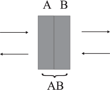
On each network, the transfer equations are written as
| (52) |
The brackets specify the network for which the matrix or field column is written. Identifying the fields according to Figure (2)
| (53) |
we deduce that the piling up process is equivalent to the product of -matrices
| (54) |
We have assumed the two networks to be in the immediate vicinity of each other but without any electronic exchange between them, which again corresponds to the assumption of thick enough layers.
III.3 Elementary networks
We now study two elementary networks, that is the traversal of an interface and the propagation over a given length inside a dielectric medium.
For the scattering at the plane interface between two media with indices and , we write the reflection and transmission amplitudes as the Fresnel scattering amplitudes LLfresnel. Reflection amplitudes are obtained from characteristic impedances defined for plane waves with polarization in each medium and from the continuity equations at the interface
| (55) |
Then the transmission amplitudes are obtained as
| (56) |
We deduce the expression of the transfer matrix
| (60) |
We now consider the process of field propagation over a propagation length inside a dielectric medium characterized by a permittivity . For this elementary network, the matrix has the simple form
| (64) |
The optical depth does not depend on the polarization.
Note that the composition is commutative within the class of interfaces or that of propagations : it corresponds to the multiplication of the parameters for interfaces and to the addition of parameters for propagations. But the composition is no longer commutative when interfaces and propagations are piled up.
III.4 Reciprocity theorem
We now prove a reciprocity theorem obeyed by arbitrary dielectric multilayers, i.e. networks obtained by piling up interfaces and propagations.
To this aim, we first remark that the ratio of the two transmission amplitudes is related to the determinant of the matrix
| (65) |
This follows from the relations (51) between and amplitudes for an arbitrary network. Then, it is clear from (54) that the determinant of is simply multiplied under composition
| (66) |
For the two kinds of elementary networks studied previously (see eqs 60-64), the determinant of is the ratio of the values of at the right and left sides of the network
| (67) |
It follows that this relation is valid for any optical network composed by piling up interfaces and propagations.
In the particular case where the network has its two ports corresponding to vacuum, which is the case for a mirror, the values of are equal on its two sides and the matrix has a unit determinant
| (68) |
Note that reciprocity corresponds to a symmetrical matrix and has to be distinguished from the spatial symmetry of the network with respect to its mediane plane which entails .
This theorem is the specific form, when the symmetry of plane mirrors is assumed, of the general reciprocity theorem demonstrated by Casimir Casimir45 as an extension to electromagnetism of Onsager’s microreversibility theorem Onsager31. We have disregarded any static magnetic field which could affect these reciprocity relations.
III.5 Slabs and multilayers
We now consider the dielectric slabs and multilayers as composed networks and we deduce their transfer and scattering amplitudes from the preceding results.
The slab is obtained by piling up a vacuum/matter interface with indices and at its left and righthand sides, propagation over a length inside matter, and a matter/vacuum interface with now and at its left and righthand sides. We denote the matrix associated with the first interface and obtain the matrix associated with the second interface as the inverse of . As a consequence of the composition law (54), the matrix associated with the slab is obtained as
| (69) |
Using the expressions (60,64) of and , we evaluate as
| (70) |
We deduce the form of the matrix which is simultaneously reciprocal () and symmetrical in the exchange of its two ports ()
| (71) |
In the limiting case of a small thickness , we find and , which means that the slab tends to become transparent. In this case indeed, the propagation can be forgotten and the two inverse interfaces have their effects cancelled by each other.
The opposite limiting case of a large thickness is often considered since it fits the usual experimental situations. More precisely, experiments are performed with metallic mirrors having a thickness much larger than the plasma wavelength. This is why the limit of a total extinction of the field through the medium is assumed in most calculations. This corresponds to the so-called ‘bulk limit’ with and in eq.(71) : the reflection amplitude is determined entirely by the first interface. Let us emphasize however that the bulk limit raises several delicate problems. First, the transmission amplitude vanishes in this limit so that the matrix is not defined, with the drawback of invalidating the general method used in the present paper. Then, the bulk limit cannot be met in the case of non absorbing media where remains a complex number with unit modulus for any value of . Even in the presence of absorption, a large value of the width does not necessarily imply a large value of the optical thickness since may go to zero at normal incidence and zero frequency, leading to a transparent slab in contrast with the results of the bulk limit. Therefore a reliable calculation must consider the experimental situation of mirrors with a large but finite thickness. In the present paper, we consider the general case of arbitrary mirrors and test the reliability of the bulk limit in the end of the calculations.
We can deal with the case of dielectric multilayers similarly. If we consider as an example the multilayer obtained by piling up a vacuum/matter interface with indices and at its left and righthand sides, propagation over a length inside the medium 1, an interface between media 1 and 2, propagation over a length inside the medium 2, and an interface between medium 2 and vacuum, its matrix is obtained as the product
| (72) | |||||
Alternatively, the same multilayer may be obtained by piling up two slabs each corresponding to one of the layers
| (73) |
In the last two equations, the indices specify the different interfaces, propagations or slabs using an obvious convention.
Since any multilayer mirror is obtained by piling up slabs connecting two vacuum ports and thus obeying the reciprocity relation , we can use a simple form of the composition law written in terms of scattering amplitudes Lambrecht97
| (74) |
For readibility, we have specified the networks by using subscripts rather than brackets. We will proceed similarly in forthcoming specific computations. Iterating this composition law, we can compute the scattering amplitudes for any dielectric multilayer. This systematic technique is quite similar to the classical computation techniques used for studying multilayers Abeles55. It is generalized to the full quantum treatment in the next section. It also leads in the following to general results constraining the variation of the Casimir force for arbitrary dielectric mirrors. It reproduces the known results for the multilayer systems which have already been studied Zhou95; Bordag01.
IV Quantum treatment of lossy mirrors
Up to now, we have performed a classical analysis which is not sufficient for the purpose of describing the scattering of vacuum fluctuations. Real mirrors consist of absorbing media which scatter incident fields to spontaneous emission modes and reciprocally scatter fluctuations from noise modes to the modes of interest. The matrix calculated previously cannot be unitary for a lossy mirror but it should be the restriction to the modes of interest of a larger matrix which includes the noise modes and obeys unitarity. In the present section, we characterize the additional fluctuations for a lossy mirror by using the corresponding ‘optical theorem’, that is also the unitarity of the larger matrix (see Barnett96; Courty00 and references therein).
We assume that the scattering restricted to the modes of interest still fulfills the symmetry of plane mirrors considered in the previous classical calculations. This amounts to neglect multiple scattering processes which could couple different modes through their coupling with noise modes. Except for this assumption, we consider arbitrary dissipative media and discuss the optical theorem in the scattering and transfer points of view. We use the latter one to deal with composition of additional fluctuations when lossy mirrors are piled up.
IV.1 Noise in the scattering approach
Should we use the previous classical equations for the quantum amplitudes, we would find that the output fields cannot obey the canonical commutators, except in the particular case of lossless mirrors. This implies that the input/output transformation for quantum field must include additional fluctuations superimposed to the classical equations
| (75) |
and are defined as in (III.1) with the quantum amplitudes in place of the classical fields , is the same matrix as previously and is a twofold column matrix describing the additional fluctuations. All these quantities depend on the quantum number which is common to all fields coupled in the scattering process.

The additional fluctuations are linear superpositions of all modes coupled to the main modes by the microscopic couplings which cause absorption. As an example, the atoms constituting a dielectric medium couple the main modes to all electromagnetic modes through spontaneous emission processes, represented symbolically by the wavy arrows on Figure 3. The stationarity assumption implies that only modes having the same frequencies are coupled. In particular, it forbids parametric couplings which could couple modes with different frequencies and ‘squeeze’ the vacuum fluctuations Reynaud90. The whole scattering matrix which takes into account all coupled field modes is unitary and this basic property makes the canonical commutation relations compatible for input and output fields. In contrast, the reduced scattering matrix containing only the classical scattering amplitudes coupling the main modes is not unitary, except in the particular case of lossless mirrors.
In order to write the unitarity property of the whole scattering matrix, it is convenient to represent the additional fluctuations by introducing auxiliary noise modes and auxiliary noise amplitudes gathered in a noise matrix
| (76) |
The components of the twofold column are defined to have the same canonical commutators as the input fields in the main modes. In fact, they are linear superpositions of the input vacuum modes responsible for the fluctuation process. They are defined up to an ambiguity : any canonical transformation of the noise modes leads to an equivalent representation of the additional fluctuations, which corresponds to a different form for the noise amplitudes while leading to the same physical results at the end of the computations.
For any of these equivalent representations, the norm matrix has the same expression determined by the optical theorem, that is the unitarity condition for the whole scattering process,
| (77) |
where is the unity matrix. This is easily proven by a direct inspection of the explicit expressions of the commutators of the output fields. The same inspection shows that noise modes corresponding to different values of are not correlated to each other. Condition (77) is made more explicit when and are developed in terms of scattering amplitudes
| (78) | |||||
More detailed discussions are presented for the case of the slab in appendix A.
The description of noise may as well be represented with the alternative representation (III.1) of the scattering process
| (79) |
The additional fluctuations are then represented in terms of the same noise modes and of a modified noise matrix
| (80) | |||||
IV.2 Noise in the transfer approach
We now present the description of additional fluctuations in the transfer approach. Performing the same manipulations as in the previous section, we transform equation (79) into
| (81) |
We thus get transfer equations with additional fluctuations described by a twofold column
| (82) |
The matrix has the same expression (47) as previously and the additional fluctuations are a linear expression of the fluctuations defined in the scattering approach. This linear relation may be written under alternative forms by using the relations (50)
| (83) |
In the scattering approach, the norm of additional fluctuations is described by matrices and which are themselves determined by the optical theorem (77) or (80). In order to translate these properties to the transfer approach, we rewrite (82) in terms of the canonical noise modes and of noise amplitudes gathered in a matrix
| (84) |
The associated norm matrix is
| (85) |
Using equations (80) and (48), we rewrite it as
| (86) |
is a diagonal matrix with two eigenvalues representing the directions of propagation of the field.
IV.3 Composition of dissipative networks
Using these tools, we now write composition laws for the fluctuations and their norms.
We start from transfer equations written for each network A and B
| (87) |
Using the identifications (53) associated with the composition law, we deduce for the composed network
| (88) |
The fluctuations are a linear superposition of fluctuations and added in A and B.
In order to obtain the composition law for the norm matrices, we develop the additional fluctuations on the canonical noise modes associated with the two elements
| (89) |
Since the noise modes associated with different elements are uncorrelated, may be rewritten in terms of new canonical noise modes and new noise amplitudes such that
| (90) | |||||
Using expression (86) of the optical theorem for both networks A and B, we deduce that the composed network AB obeys the same relation
| (91) | |||||
Equivalently, the matrix of the composed network AB obeys the optical theorem (77) as soon as the two networks A and B do.
IV.4 Resonance for cavity fields
We have studied the scattering or, equivalently, the lefthand/righthand transfer of fields by a composed network AB. We want now to characterize the properties of the fields inside the cavity formed between A and B. This problem will play a key role in the evaluation of the Casimir force (see next section).

The situation is illustrated by Figure 4 which, in contrast to Figure 2, keeps the trace of the intracavity fields. In algebraic terms, the cavity fields are defined by rewriting the identifications (53) as
| (92) |
From now on, we drop the label for the composed network and use subscripts for the networks A and B.
In order to express the cavity fields in terms of the input modes and additional fluctuations, we first write the cavity fields in terms of the righthand ones
| (93) |
We then identify the two components of as
| (94) |
Using the expression of in terms of and the composition law (88) for , we deduce
| (95) |
As already explained, the unitarity of scattering entails that the output fields have the same commutators as the input ones. But this is not the case for the cavity fields which have their commutators determined by the matrix
| (96) |
Expanding this quadratic form and using the composition law (90), we rewrite as
| (97) | |||||
Using relation (86) for the three networks A, B and AB, we obtain a simpler expression after a few rearrangements
| (98) |
We now proceed to explicit calculations of these matrices. We note that where is the transmission amplitude of the network AB and deduce
| (99) |
is simply the inverse of the transfer amplitude associated with the network AB (see eq.51) and the latter is deduced from the composition law (54)
| (100) |
Then, the transfer amplitudes of the networks A and B may be substituted by the associated scattering amplitudes, leading to
| (101) |
Collecting these results and proceeding to slight rearrangements, we finally get
In the following we will use the diagonal terms of the matrix to evaluate the Casimir force.
IV.5 Scattering on a Fabry-Perot cavity
In order to prepare the evaluation of the Casimir force, we generalize the preceding expression to the case of the Fabry-Perot cavity containing a zone of field propagation between the two mirrors M1 and M2 (see Figure 5).

The distance between the two mirrors is denoted and the cavity fields are defined at an arbitrary position inside the cavity, say at distances from M1 and from M2 with . In these conditions, the study of the Fabry-Perot cavity is reduced to the problem studied in the preceding subsection through the following identifications : the network A contains the mirror M1 and the propagation L1 with while the network B contains the propagation L2 and the mirror M2 with . The transfer amplitudes for the networks A and B are derived from those corresponding to M1 and M2 and from phase factors corresponding to the propagations L1 and L2
| (108) |
We have labeled the amplitudes for the mirrors M1 and M2 with mere indices 1 and 2; is defined in vacuum. These results entail that the reflection amplitudes and are seen from a point inside the cavity as the product of phase factors by the reflection amplitudes and seen from a point in the immediate vicinity of M1 and M2.
We then deduce the scattering amplitudes for the whole cavity
| (109) |
and the expression of
The diagonal terms in the matrix coincide with the Airy function
| (116) |
This result will play the central role in the derivation of the Casimir force in the next section. It means that the commutators of the intracavity fields are not the same as those of the input or output fields. They correspond to a spectral density modified through a multiplication by the Airy function . This is the basic property used in Cavity Quantum ElectroDynamics Haroche84.
It is clear from the present derivation that this result has a quite general status : it is obtained for any inner field in any composed network, assuming the symmetry of plane mirrors. This property was already known for non absorbing mirrors Jaekel91 and for lossy mirrors symmetrical with respect to their mediane plane Barnett98. The present derivation proves that it is also valid for arbitrary dielectric multilayers with dissipation. The final result only depends on the reflection amplitudes and of the mirrors as they are seen from the inner side of the cavity. The reflection amplitudes seen from the outer side and the transmission amplitudes do not appear in expressions (IV.5,116). This can be interpreted as resulting from the unitarity of the whole scattering processes.
V Casimir force between real mirrors
We may now deal with the radiation pressure of vacuum fields on the mirrors of a Fabry-Perot cavity. We show that the resulting Casimir force is a regular integral which can be written over real or imaginary frequencies. We then derive general constraints obeyed by the Casimir force for arbitrary dielectric mirrors.
V.1 Vacuum radiation pressure
If we first consider a mirror isolated in vacuum, the radiation pressure is obtained by adding the contributions of the 4 fields coupled in the scattering process
| (117) |
The identification of these fields is given by Figure (1). We have developed the sum over and kept the symbol to represent the quantum numbers . We assume that the whole system is in vacuum, that is at zero temperature, so that the anticommutators of input fields are given by relation (8). Since the commutators are the same for the output and input fields, the vacuum radiation pressure vanishes in the case of an isolated mirror. In other words, the two sides of the mirror play equivalent roles so that no mean force can appear.
When we consider two mirrors forming a Fabry-Perot cavity, the two sides of a given mirror are no longer equivalent since one is an inner side and the other an outer side. It follows that the compensation observed for an isolated mirror does no longer hold, resulting in the appearance of the Casimir force. In order to evaluate the force, we write the mean radiation pressures and on mirrors M1 and M2 (see Figure 5)
| (118) |
For the same reasons as previously, the field anticommutators are given by (8) for input and output fields. For intracavity fields, they are multiplied by the Airy function (116) like the commutators
| (119) | |||||
As shown in the previous section, these expressions do not depend on the position inside the cavity where the cavity fields are defined. We finally deduce the mean radiation pressures on mirrors M1 and M2
| (120) | |||||
At this point, it is worth emphasizing that we have assumed equilibrium at zero temperature for the whole system : not only the input fields but also any fluctuations associated with loss mechanisms inside the mirrors correspond to zero-point fluctuations, whatever their microscopic origin may be. Otherwise, the expression of the force discussed in the following would be affected.
The pressures have opposite values on the two mirrors M1 and M2. This entails that the global force exerted by vacuum upon the cavity vanishes, in consistency with the translational invariance of vacuum. In the following, we denote the Casimir force calculated for M1 when considering the limit of a large area
| (121) |
The sign conventions used here are such that the positive value obtained below for corresponds to an attraction of the two mirrors to each other.
V.2 The force as an integral over real frequencies
We now perform a change of variable to rewrite the summation symbol as specified in (5)
| (122) | |||||
We will now specify the domain of integration for .
Up to now, we have discussed the scattering for ordinary waves which freely propagate in vacuum and correspond to frequencies larger than the bound fixed by the norm of the transverse wavevector. But we must also take into account the contribution of evanescent waves which correspond to frequencies smaller than . These waves are fed by the additional fluctuations coming from the noise lines into the dielectric medium and propagating with an incidence angle larger than the limit angle. They are thus transformed at the interface into evanescent waves decreasing exponentially when the distance from the interface increases. As is well known BWevanescent, the properties of these evanescent waves are conveniently described through an analytical continuation of those of ordinary waves. This analytical continuation can only be dealt with in terms of functions having a well defined analyticity behaviour. This is not the case for the Airy function but we know that this function is the sum (116) of parts having well defined analyticity properties
| (123) |
is the ‘open loop function’ corresponding to one round trip of the field inside the cavity and defined as the product of the reflection amplitudes and of the two mirrors and of the propagation phaseshift ; it is an analytical function in the physical domain of complex frequencies with the branch of the square root chosen so that . Since the transverse wavevector is spectator throughout the whole scattering process, analyticity is defined with fixed.
Then, is the ‘closed loop function’ built up on the open loop function . It is also an analytical function, thanks to analyticity of the open loop and to a stability property which has a natural interpretation : the system formed by the Fabry-Perot cavity and the vacuum fluctuations is stable because neither the mirrors nor the vacuum would have the ability to sustain an oscillation. In some cases, the stability can be derived from a more stringent passivity property Lambrecht97 which may essentially be written . However, the passivity property is sometimes too stringent to be obeyed by real mirrors (see more detailed discussions in appendix B). In any case, the stability property, i.e. the absence of self sustained oscillations, is sufficient for the present derivation of the Casimir force.
We are now able to give more precise specifications of the domain of integration in (122). Using the decomposition (123), we write the contribution of ordinary waves to this integral as the sum of two conjugated expressions
| (124) |
The integral is built on the retarded function which may be extended through an analytical continuation from the sector of ordinary waves to that of evanescent waves. The contribution of evanescent waves to the force is thus obtained as
| (125) |
The final expression of the Casimir force is the sum of the contributions of ordinary and evanescent waves that is also the integral over the whole axis of real frequencies
| (126) |
As far as ordinary waves are concerned, this corresponds to the intuitive picture where the Casimir force results from the radiation pressure of vacuum fluctuations filtered by the cavity Jaekel91. The contribution of evanescent waves is but the extension of the domain of integration to the whole real axis with the cavity response function extended through an analytical continuation. In the evanescent sector, the cavity function is written in terms of reflection amplitudes calculated for evanescent waves and exponential factors corresponding to evanescent propagation through the cavity. This means that it describes the ‘frustration’ of total reflection on one mirror due to the presence of the other. This explains why the radiation pressure of evanescent waves is not identical on the two sides of a given mirror and, therefore, how evanescent waves have a non null contribution to the Casimir force.
V.3 The force as an integral over imaginary frequencies
Using the Cauchy theorem, we now rewrite the Casimir force (126) as an integral over the axis of imaginary frequencies.

Since is analytical in the domain , its integral over a closed contour lying in this domain has to vanish. We choose the contour drawn on Figure 6 which consists of the positive part of the real axis including ordinary (Co) and evanescent (Ce) waves, a quarter of circle C∞ with a very large radius and, finally, the imaginary axis Ci run from infinity to zero. Now the function goes to zero for large values of the frequency, as a consequence of transparency at high frequency, a property certainly valid for any realistic model of optical mirror. Thanks to this property, the contribution to the integral of C∞ vanishes. We then deduce that the integrals over the real axis and over the imaginary axis are equal.
We thus get a new expression of the force as an integral over imaginary frequencies , that is also as an integral over real values of ,
| (127) | |||||
We have used the fact that is real, so that is simply equal to . This property is less obvious, but also true, with written as an integral over real frequencies. We wish to emphasize more generally that expression (127) is mathematically equivalent to (126). The former expression is closer to the physical intuition whereas the latter is better adapted to explicit computations of the force.
Expression (127) gives the Casimir force between real mirrors described by arbitrary frequency dependent reflection amplitudes. It is a regular integral as soon as these amplitudes obey the physical assumptions used in the derivation : causality, unitarity and high frequency transparency for each mirror, stability of the system formed by the two mirrors and the scattered vacuum fields. The demonstration holds for dissipative mirrors and not only for lossless ones.
The limit of perfect mirrors is obtained in expression (127) by letting the reflection amplitudes go to unity, which leads to the Casimir formula (1). This can be considered as an alternative demonstration of the Casimir formula without any reference to a renormalization or regularization technique. Basically, the properties of real mirrors, in particular their high frequency transparency, are sufficient to provide a regular expression of the force, as it was guessed a long time ago by Casimir Casimir48.
As a simple model of the mirrors used in the experiments, let us consider a metallic slab with a large width, that is a width larger than a few plasma wavelengthes. We use expression (127) of the force written as an integral over imaginary values of the frequencies (, real). Hence, the phase factor corresponding to one round trip inside the slab is a decreasing exponential with a real exponent . For the plasma model (14), is given by and it is larger than for all values of and . When relaxation is taken into account, this is still the case except in a very narrow domain with values of and both close to zero. This domain has a negligible contribution to the integral (127) and it follows that the reflection amplitude of the slab may be replaced by the limiting expression obtained for the bulk. One thus recovers the Lifshitz expression for the Casimir force Lifshitz56 which is widely used for comparing experimental results with theoretical expectations Bordag01.
V.4 Constraints on the force
We now deduce general constraints which invalidate proposals made for tayloring the Casimir force at will by using specially designed mirrors Iacopini93; Ford93. This generalizes to 3D space the results obtained for 1D space in Lambrecht97 to which the reader is referred for further discussions.
Expression (127) is an integral over the axis of imaginary frequencies essentially determined by the reflection amplitudes and for real. These amplitudes always have a modulus smaller than unity, for arbitrary dielectric multilayers (see appendix C). They are negative for arbitrary dielectric slabs (see appendix A) and we deduce from the composition law (74) that this is still the case for arbitrary dielectric multilayers. It follows that the product of the reflection amplitudes of the two mirrors is always positive with a modulus smaller than unity
| (128) |
From this, we deduce first that the Casimir force has an absolute value smaller than the value (1) reached for perfect mirrors and that it remains attractive
| (129) |
We also derive that the Casimir force decreases as a function of the length
| (130) |
This means that the properties obeyed by real mirrors strongly constrain the possible variation of the Casimir force, contrarily to what might have been expected at first sight Iacopini93; Ford93.
Note that we have considered mirrors used in the experiments which have electric permittivity but no magnetic permeability. Different results would be obtained with magnetic mirrors, precisely with one of the mirrors dominated by electric response and the other one by magnetic response. The product of the two reflection amplitudes would indeed be negative in this case and the Casimir force repulsive Boyer74; Kupiszewska93; Alves00; Kenneth02.
VI Conclusion
We have presented a derivation of the Casimir force between lossy mirrors characterized by arbitrary frequency dependent reflection amplitudes, in the Casimir geometry where the cavity is made with two parallel plane mirrors.
We have shown how mirrors and cavities may be dealt with by using a quantum theory of optical networks. We have deduced the additional fluctuations accompanying dissipation from expressions of the optical theorem adapted to quantum network theory. The optical theorem is equivalent to the unitarity of the whole scattering process which couples the modes of interest and the noise modes and it ensures that the quantum commutators of the output fields are the same as those of the input fields. The situation is different for the cavity fields which do not freely propagate. We have given a general proof of a theorem previously demonstrated in particular cases Jaekel91; Barnett98 which states that the modification of the commutators is determined by the usual Airy function, that is the spectral density associated with the Fabry-Perot cavity. For arbitrary lossy mirrors, the spectral density is determined by the reflection amplitudes as they are seen by the intracavity fields. It determines the radiation pressure exerted by vacuum fluctuations upon the mirrors with repulsive and attractive contributions associated respectively with resonant or antiresonant frequencies. The Casimir force is then obtained as an integral over the whole axis of real frequencies, including the contribution of evanescent waves besides that of ordinary waves. It is equivalently expressed as an integral over imaginary frequencies. The derivation only uses a few general assumptions certainly valid for real optical mirrors, namely causality, unitarity, high-frequency transparency for each mirror and stability of the compound cavity-vacuum system. It leads to a finite result without any further reference to a regularization technique Jaekel91.
The formula obtained in the present paper for the Casimir force was already known Jaekel91 but its scope of validity is widened by the present demonstration. It has been used to discuss the effect of imperfect reflection for the metallic mirrors used in the experiments. Different descriptions of the optical response of metals have been used, from the crude application of the plasma model (14) to a more complete characterization of the dielectric constant derived from tabulated optical data and dispersion relations. This kind of calculations, discussed in great detail for the mirrors corresponding to the recent experiments (see for example Lambrecht00), has not been reproduced here. Instead, we have presented general results valid for any real mirrors obeying the physical properties already evoked and shown that they strongly constrain the variation of the Casimir force.
In the present paper, we have restricted our attention on the limit of zero temperature although our work was partly motivated by a recent polemical discussion of the effect of temperature on the Casimir force between real mirrors Bostrom00; Svetovoy00; Bordag00; Lamoreaux01c; Sernelius01r; Sernelius01c; Bordag01r; Klimchitskaya01; Bezerra02; Lamoreaux02. Since contradictory results may have raised doubts about the validity and consistency of various derivations of the Casimir force, we have considered it was important to come back to the first principles in this derivation. This has been done in the present paper for the case of zero temperature. A follow-on publication will show how to include the effect of thermal fluctuations in the treatment in order to obtain an expression free from ambiguities for the Casimir force between arbitrary lossy mirrors at non zero temperatures.
Appendix A The dielectric slab
In this appendix, we discuss in more detail the specific case of the dielectric slab. We consider lossy as well as lossless slabs.
For a lossless dielectric medium, the permittivity is real at real frequencies. For ordinary waves, and are purely imaginary, so that the impedance ratios are real for both polarizations. Hence is real () and purely imaginary () so that the scattering amplitudes (71) are read as
| (131) | |||||
The sum of the squared amplitudes is unity while the reflexion and transmission amplitudes are in quadrature to each other , which means that is a unitary matrix, as it was expected for a lossless mirror. This implies that the reflection amplitude has a modulus smaller than unity . This property also holds for lossy mirrors thanks to positivity of dissipation (see appendix C).
Unitarity is defined without ambiguity only in the case of ordinary waves. For a lossless slab and evanescent waves, is real - it is just the inverse of the penetration length of evanescent wave in vacuum - whereas remains purely imaginary. Hence as well as are purely imaginary and it is no longer possible to obtain general bounds for the scattering amplitudes
| (132) |
In particular, does not remain always smaller than 1 (see more explicit discussions in appendix B with different results for the TE and TM polarizations).
For imaginary frequencies finally, and are positive real numbers, for lossy as well as lossless slabs. In this case, general bounds are easily obtained for the amplitudes
| (133) |
The fact that is negative with a modulus smaller than unity plays an important role in the derivation of constraints on the Casimir force.
Interesting results are also obtained for the eigenvalues of the matrix, which have a simple form since the slab is symmetrical in the exchange of its two ports. In the sector of ordinary waves, unitarity (77) has a simple form in terms of and of the similar quantities defined on the noise matrix
| (134) |
For the lossless slab, have a unit modulus and vanish. For a lossy slab, we have
| (135) |
This can be considered as a consequence of (134) with . Equivalently, it can be considered that unitarity (134) fixes the modulus of when the modulus of is known.
Condition (135) will be found in appendix C to express a passivity property for the slab, here for ordinary waves. This property still holds in the sector of imaginary frequencies, as a consequence of (133) and of the following inequalities obeyed for all positive real numbers and
| (136) |
Using the terms of appendix C, this means that the domain of passivity always includes the sectors of ordinary waves and imaginary frequencies, in the case of a dielectric slab. However, it does not necessarily include the sector of evanescent waves (see appendix B).
Appendix B The sector of evanescent waves
Ordinary waves correspond to frequencies and real wavevectors whereas evanescent waves correspond to frequencies and imaginary values of . Causal scattering amplitudes can be extended from ordinary to evanescent waves, by an analytical continuation through the physical domain of complex frequencies with and . The ‘energy conditions’ which bear on quadratic forms are not necessarily preserved in this process.
In order to illustrate the idea, let us consider the reflection amplitude (55) at the interface between vacuum () and a lossless dielectric medium ( real for real). In the sector of evanescent waves, is imaginary and real, so that and are complex numbers with a unit modulus, that is also pure dephasings corresponding to the phenomenon of total reflection. Meanwhile, the transmission amplitudes differ from zero, which describes how evanescent waves in vacuum are fed by the fields coming from the dielectric medium with an incidence angle larger than the limit angle. In these conditions, it is clear that the condition fails.
For the TE polarization, it turns out that
| (137) |
in the evanescent sector at the interface between vacuum and any dielectric medium. This property is always true in the sectors of ordinary waves and imaginary frequencies for an arbitrary mirror (see the appendices A and C). Using high frequency transparency, it follows from the Phragmén-Lindelöf theorem Phragmen that inequality (137) holds in the whole physical domain in the complex plane. This ensures that the closed loop function is analytic and, in particular, has no pole in the domain . In other words, since the open loop gain is smaller than unity, the closed loop cannot reach the oscillation threshold, leading to the stability property used in the derivation of the Casimir force.
Although it seems quite natural, this argument is not valid in the general case. For metallic mirrors for example, the condition is violated in the evanescent sector for TM modes. The reflection amplitude is even known to reach large resonant values at the plasmon resonances Barton79. Of course, this does not prevent the stability property to be fulfilled : the Fabry-Perot cavity is in this case a stable closed loop built on an open loop exceeding the unit modulus but with a phase such that the oscillation threshold is not reached.
We stress again that the stability property is necessary in the derivation of the Casimir force since it entails that the closed loop function is properly defined in the evanescent sector. When the more stringent property is also obeyed, it follows from expression (123) that the Airy function, which has been defined with the significance of a positive spectral density on ordinary waves, remains positive in the evanescent sector. When the property fails, the Airy function can no longer be thought of as a spectral density in the whole physical domain, but this does not invalidate the derivation of the Casimir force.
Appendix C The domain of passivity
In this appendix, we discuss the related but not identical properties corresponding to positivity of dissipation and passivity.
We consider an arbitrary mirror, that is a reciprocal network connecting two vacuum ports. For ordinary waves, we define the power dissipated by the mirror
| (138) | |||||
where we have introduced row vectors conjugated to the column vectors
| (139) |
This power is positive as a consequence of unitarity
| (140) | |||||
which corresponds to the positivity of the matrix
| (141) |
where represents arbitrary input fields. Positivity can also be expressed in terms of the eigenvalues of
| (142) |
These eigenvalues are always real and positivity of dissipation is equivalent to the fact that they are smaller than unity
| (143) |
Passivity is a property directly related to positivity of dissipation but defined more generally for complex frequencies in the physical domain. In order to discuss it, we extend the matrix from the sector of ordinary waves through the analytical continuation already discussed. We extend similarly, with the complex conjugation cautiously defined since it involves complex frequencies : conjugation corresponds to and and it preserves the physical domain ; the derivations performed for an amplitude in the domain are thus translated to similar derivations for the conjugated amplitude in the quarter plane .
Then, the domain of passivity of is defined by the domain of for which is a positive matrix (eq.141) that is also for which the eigenvalues of are smaller than unity (eq.143). An important feature of this property is that it is stable under composition : when two networks A and B are piled up as in Figure 2, the quadratic forms appearing in (141) simply add up so that passivity of the network AB follows from passivity of the two networks A and B. This is a special case of a general theorem Meixner which states that networks built up with passive elements are passive.
Passivity means that the eigenvalues of the matrix are both positive, which is equivalent to the following inequalities
| (144) |
It may be written in terms of the scattering amplitudes
| (145) |
Passivity implies that the scattering amplitudes have a modulus smaller than unity
| (146) |
Conversely, the latter conditions are necessary but not sufficient for passivity.
For a mirror symmetrical in the exchange of its two ports, a slab for example, the passivity conditions take the simple form . The results of appendix A thus entail that the domain of passivity always includes the sectors of ordinary waves and imaginary frequencies, for arbitrary slabs (eq.135). Using the stability of passivity under composition, we deduce that this is also the case for arbitrary multilayers. It follows that the reflection amplitudes always have a modulus smaller than unity for imaginary frequencies ( real)
| (147) |
Acknowledgements.
Thanks are due to Gabriel Barton and Marc-Thierry Jaekel for their helpful comments.References
- (1) H.B.G. Casimir, Proc. K. Ned. Akad. Wet. 51, 793 (1948).
- (2) B.V. Deriagin and I.I. Abrikosova, Sov. Phys. JETP 3, 819 (1957).
- (3) M.J. Sparnaay, Physica XXIV, 751 (1957).
- (4) D. Tabor and R.H.S. Winterton, Nature 219, 1120 (1968).
- (5) W. Black, J. G. V. De Jong, J.Th.G. Overbeek and M.J. Sparnaay, Trans. Faraday Soc. 56, 1597 (1968).
- (6) E.S. Sabisky and C.H. Anderson, Phys. Rev. A 7, 790 (1973).
- (7) M.J. Sparnaay, in Physics in the Making eds Sarlemijn A. and Sparnaay M.J., 235 (North-Holland, 1989) and references therein.
- (8) P.W. Milonni, The quantum vacuum (Academic, 1994).
- (9) V.M. Mostepanenko and N.N. Trunov, The Casimir effect and its applications (Clarendon, 1997).
- (10) S.K. Lamoreaux, Phys. Rev. Lett. 78, 5 (1997); Erratum in Phys. Rev. Lett. 81, 5475 (1998).
- (11) U. Mohideen and A. Roy, Phys. Rev. Lett. 81, 4549 (1998).
- (12) A. Roy, C. Lin, and U. Mohideen, Phys. Rev. D 60, 111101 (1999).
- (13) B.W. Harris, F. Chen and U. Mohideen, Phys. Rev. A 62, 052109 (2000).
- (14) Th. Ederth, Phys. Rev. A 62, 062104 (2000).
- (15) H.B. Chan, V.A. Aksyuk, R.N. Kleiman, D.J. Bishop and F. Capasso, Science 291, 1941 (2001).
- (16) H.B. Chan, V.A. Aksyuk, R.N. Kleiman, D.J. Bishop and F. Capasso, Phys. Rev. Lett. 87, 211801 (2001).
- (17) E. Buks and M.L. Roukes, EuroPhys. Lett. 54, 220 (2001).
- (18) G. Bressi, G. Carugno, R. Onofrio and G. Ruoso, Phys. Rev. Lett. 88, 041804 (2002).
- (19) M. Bordag, U. Mohideen and V.M. Mostepanenko, Phys. Rep. 353, 1 (2001).
- (20) A. Lambrecht and S. Reynaud, Séminaire Poincaré 1, 107 (2002).
- (21) S. Reynaud, A. Lambrecht, C. Genet and M.T. Jaekel, C. R. Acad. Sci. Paris IV-2, 1287 (2001).
- (22) C. Genet, A. Lambrecht and S. Reynaud, preprint (2002) arXiv:quant-ph/0210173 and references therein.
- (23) G. Carugno, Z. Fontana, R. Onofrio and C. Rizzo, Phys. Rev. D 55, 6591 (1997).
- (24) E. Fischbach and C. Talmadge, The Search for Non Newtonian Gravity (AIP Press/Springer Verlag, 1998).
- (25) M. Bordag, B. Geyer, G.L. Klimchitskaya and V.M. Mostepanenko, Phys. Rev. D 60, 055004 (1999).
- (26) E. Fischbach and D.E. Krause, Phys. Rev. Lett. 82, 4753 (1999).
- (27) J.C. Long, H.W. Chan and J.C. Price, Nucl. Phys. B 539, 23 (1999).
- (28) C.D. Hoyle et al, Phys. Rev. Lett. 86, 1418 (2001).
- (29) E.G. Adelberger et al, preprint (2002) arXiv:hep-ex/0202008.
- (30) J.C. Long et al, preprint (2002) arXiv:hep-ph/0210004.
- (31) A. Lambrecht and S. Reynaud, Eur. Phys. J. D 8, 309 (2000).
- (32) M. Boström and Bo E. Sernelius, Phys. Rev. Lett. 84, 4757 (2000).
- (33) V.B. Svetovoy and M.V. Lokhanin, Mod. Phys. Lett. A 15, 1013 and 1437 (2000); Phys. Lett. A 280, 177 (2001).
- (34) M. Bordag, B. Geyer, G.L. Klimchitskaya and V.M. Mostepanenko, Phys. Rev. Lett. 85, 503 (2000).
- (35) S.K. Lamoreaux, Comment on Bostrom00, Phys. Rev. Lett. 87, 139101 (2001).
- (36) Bo E. Sernelius, Reply to Lamoreaux01c, Phys. Rev. Lett. 87, 139102 (2001).
- (37) Bo E. Sernelius and M. Boström, Comment on Bordag00, Phys. Rev. Lett. 87, 259101 (2001).
- (38) M. Bordag, B. Geyer, G.L. Klimchitskaya and V.M. Mostepanenko, Reply to Sernelius01c, Phys. Rev. Lett. 87, 259102 (2001).
- (39) G.L. Klimchitskaya and V.M. Mostepanenko, Phys. Rev. A 63, 062108 (2001).
- (40) V.B. Bezerra, G.L. Klimchitskaya and V.M. Mostepanenko, Phys. Rev. A 65, 052113 (2002).
- (41) J.R. Torgerson and S.K. Lamoreaux, preprint (2002) arXiv:quant-ph/0208042.
- (42) M.T. Jaekel and S. Reynaud, J. Physique I-1, 1395 (1991); also available as eprint arXiv:quant-ph/0101067.
- (43) S.M. Barnett, J. Jeffers, A. Gatti and R. Loudon, Phys. Rev. A 57, 2134 (1998).
- (44) J. Meixner, J. of Math. Phys. 4, 154 (1963); J. Meixner in Statistical mechanics of equilibrium and non-equilibrium ed. J. Meixner, 52 (North Holland, 1965); J. Meixner, Acta Phys. Polonica 27, 113 (1965).
- (45) E.M. Lifshitz, Sov. Phys. JETP 2, 73 (1956).
- (46) E.M. Lifshitz and L.P. Pitaevskii, Landau and Lifshitz Course of Theoretical Physics: Statistical Physics Part 2 (Butterworth-Heinemann, 1980) ch VIII.
- (47) E. Iacopini, Phys. Rev. A 48, 129 (1993).
- (48) L.H. Ford, Phys. Rev. A 48, 2962 (1993).
- (49) A. Lambrecht, M.T. Jaekel and S. Reynaud, Phys. Lett. A 225, 188 (1997).
- (50) C. Cohen-Tannoudji, J. Dupont-Roc and G. Grynberg, Introduction à l’ElectroDynamique Quantique (InterEditions/CNRS, 1987).
- (51) L. Landau, E.M. Lifshitz and L.P. Pitaevskii, Landau and Lifshitz Course of Theoretical Physics: Electrodynamics in Continuous Media (Butterworth-Heinemann, 1980) §79 and §82.
- (52) See §86 in LLcausality.
- (53) M. Born and E. Wolf, Principles of Optics (Cambridge University Press, 1999) §1.5.4.
- (54) H.B.G. Casimir, Rev. of Mod. Phys. 17, 343 (1945).
- (55) L. Onsager, Phys. Rev. 37, 405 (1931), 38, 2265 (1931).
- (56) F. Abelès, Ann. d. Physique 5, 611 (1955).
- (57) F. Zhou and L. Spruch, Phys. Rev. A 52, 297 (1995).
- (58) S.M. Barnett, C.R. Gilson, B. Huttner and N. Imoto, Phys. Rev. Lett. 77, 1739 (1996).
- (59) J.M. Courty, F. Grassia and S. Reynaud, in Noise, Oscillators and Algebraic Randomness, ed. M. Planat (Springer, 2000) p.71.
- (60) S. Reynaud, Ann. Physique 15, 63 (1990).
- (61) S. Haroche, in New Trends in Atomic Physics G.Grynberg and R.Stora eds., 193 (North Holland, 1984).
- (62) T.H. Boyer, Phys. Rev. A 9, 2078 (1974).
- (63) D. Kupiszewska, J. of Mod. Opt. 40, 517 (1993).
- (64) D.T. Alves, C. Farina and A.C. Tort, Phys. Rev. A 61, 034102 (2000).
- (65) O. Kenneth, I. Klich, A. Mann and M. Revzen, Phys. Rev. Lett. 89, 033001 (2002).
- (66) H.M. Nussenzveig, Causality and dispersion relations (Academic Press, New York, 1972).
- (67) G. Barton, Rep. Prog. Phys. 42, 65 (1979).