Entanglement generation and Hamiltonian simulation in Continuous-Variable Systems
Abstract
Several recent experiments have demonstrated the promise of atomic ensembles for quantum teleportation and quantum memory. In these cases the collective internal state of the atoms is well described by continuous variables and the interaction with the optical field () by a quadratic Hamiltonian . We show how this interaction can be used optimally to create entanglement and squeezing. We derive conditions for the efficient simulation of quadratic Hamiltonians and the engineering of all Gaussian operations and states.
pacs
03.67.-aI Introduction
After the first experiments Furusawa et al. 1998 on quantum teleportation using two–mode squeezed states Vaidman 1994; Braunstein and Kimble 1998, as well as those Hald et al. 1999; Julsgaard et al. 2000; Kuzmich et al. 2000 dealing with entanglement in atomic ensembles Kuzmich and Polzik 2000; Duan et al. 2000a, a significant amount of work has been devoted to develop a quantum information theory of continuous variable systems. So far, most of the theoretical work has focused on the entanglement properties of the quantum states involved in all these experiments, the so–called Gaussian states. Some examples of the achievements in this field are the following. The problem of qualifying entanglement has been solved in the general bipartite setting Duan et al. 2000b; Simon 2000; Werner and Wolf 2001; Giedke et al. 2001a and in the three mode case Giedke et al. 2001b. The distillation problem has also been answered in the general case Giedke et al. 2001c, as well as in the case in which the class of allowed operations is restricted to those that conserve the Gaussian form Giedke and Cirac 2002; Eisert et al. 2002; Fiurášek 2002. In contrast to all this theoretical work on (the static) entanglement properties of Gaussian states, very few results Thomsen et al. 2002; Bouchoule and Mølmer 2002; Di Lisi and Mølmer 2002; Berry and Sanders 2002 have been obtained on the dynamics of entanglement on these systems, i.e., on how to use the interactions provided by the physical set–ups in order to entangle the systems in the most efficient way. This paper provides a rather complete theory of the dynamics of entanglement in these experimental settings.
The dynamics of entanglement has been recently analyzed in systems of two or more qubits Dür et al. 2001; Kraus and Cirac 2001; Zanardi et al. 2000; Dodd et al. 2002; Wocjan et al. 2002; Nielsen et al. 2001; Bennett et al. 2002a; Leifer et al. 2002. In that case one distinguishes between two scenarios. In the first one Dür et al. 2001; Zanardi et al. 2000, the interaction between the qubits is described by a Hamiltonian . The goal is to determine the sequence of local gates for which the increase of entanglement after some small (infinitesimal) time is maximal for a given initial state. In the second one Kraus and Cirac 2001; Dodd et al. 2002; Leifer et al. 2002, the interaction is given in terms of a non–local gate, which can be applied only once. Apart from its fundamental interest, these studies give some practical ways of creating entanglement in the most efficient way and may become relevant in several experimental situations. Another interesting and related problem is the one of Hamiltonian and gate simulation Vidal and Cirac 2002; Bennett et al. 2002b; Vidal et al. 2002; Hammerer et al. 2002. Here, one assumes that the two qubits interact via some given Hamiltonian and the goal is to determine a sequence of local instantaneous gates in order to obtain in minimal time either a complete time-evolution generated by some other Hamiltonian [Hamiltonian simulation] or some desired unitary gate (gate engineering).
In the present paper we analyze all these problems for two–mode pure Gaussian states and interaction Hamiltonians which preserve the Gaussian character. We also study the generation of squeezing, since although it has no counterpart in the qubit case, it is a valuable resource in present experiments Wolf et al. 2002. Given the fact that we touch on several different topics and therefore develop different mathematical tools, we have decided to write a section which explains in detail the different problems we consider and the corresponding results. In the following sections we give detailed derivations of these results.
We stress the fact that the problems studied here are all motivated by the experimental situation in which light gets entangled with an atomic ensemble via a Kerr–like interaction Kuzmich et al. 1998; Mølmer 1999; Polzik 1999; Duan et al. 2000a. We expect that the techniques developed in this paper can be easily extended to address other related problems, like the one of entangling two atomic ensembles using light.
The paper is organized as follows: The section Sec. II should be considered as a survey of the results presented in the paper. In Section Sec. III we show which Hamiltonians can be simulated using a given interaction and how to do so optimally. We also show that, in fact, any general Gaussian operation can be generated in the considered set–up. In Section Sec. IV.2 we determine the optimal rate of entanglement generation as well as of squeezing generation for arbitrary input states. Finally, in Section Sec. IV.3 we give an optimal entanglement generation scheme for finite times, starting out from a product (unsqueezed) state.
II Overview
This section gives an overview of the content of this paper and it is composed of three subsections. In the first one, we explain the physical set-up that we are going to analyze. In the second one we collect the main definitions used thereafter. In the third section we give the main results of the paper without proving them. For the detailed derivations we refer the reader to the following sections.
II.1 Setup
We consider a continuous variable system composed of two one–mode systems coupled via some interaction Hamiltonian. The goal is to analyze which kind of evolutions we can achieve with such an interaction if certain instantaneous local operations can be applied at will. In particular, we study optimal methods of creating or increasing the entanglement shared by the two modes.
The interaction Hamiltonian has the general form
| (1) |
where and are real parameters, and and are canonical operators for the first and second mode, respectively 11 1 Note that the Hamiltonians that we are considering here are not semi-bounded. However, this is not a problem since we are always considering initial states and times for which the real Hamiltonian can be locally approximated by these Hamiltonians.. We use dimensionless units throughout the paper. We assume that local operations, generated by the Hamiltonians
| (2) |
can be applied instantaneously, where is a real number that can be tuned at will ††footnotemark: . These operations can neither change the entanglement nor the squeezing present in the state. Lastly, we assume that the initial state is pure and Gaussian.
Our choice of the Hamiltonian interaction as well as the instantaneous local operations is motivated by current experiments with atomic ensembles Schori et al. 2002; Julsgaard et al. 2000; Kuzmich et al. 2000; Hald et al. 1999. In particular, to those set-ups in which an atomic ensemble interacts with two modes of the electromagnetic field 22 2 This is the case if the atomic ensemble is embedded in a ring cavity, for example. Note that for optically thick samples, the description may also be valid in free space. with different polarizations Kuzmich et al. 1998; Kuzmich and Polzik 2000; Duan et al. 2000c; Duan et al. 2002. If the atoms are sufficiently polarized along some given direction (say ) we can replace the total angular momentum operators describing the internal state of the atoms by canonical operators. That is (if the involved levels have spin ), , , , with (), and where is the number of atoms. This approximation is valid as long as for all times Arecchi et al. 1972. Similarly, if the electromagnetic field is sufficiently polarized along some direction, we can substitute the Stokes operators by canonical ones, and Schnabel et al. 2002.
For some atomic structures and off-resonant interactions, the Hamiltonian describing the interaction between the atomic ensemble and the light can be written as Kuzmich et al. 1998
| (3) |
which is a particular case of Eq. (1); in the following we will put the coupling constant when referring to . In the same scenario, simple and fast local operations can be performed on the atoms and the electromagnetic field. For example, a magnetic field or a polarizer gives rise to the local Hamiltonians Eq. (2). Since the interaction between atoms and light is typically weak, with moderate magnetic fields the operations generated locally can be regarded as instantaneous. On the other hand, if the atoms and the light are completely polarized, the corresponding state in terms of our continuous variable description is the tensor product of two vacuum states, in particular it is a pure Gaussian state.
We emphasize that even though we have motivated our choices with some particular physical set-up, our description is applicable to other physical situations and our results apply to the general interaction Hamiltonian Eq. (1). In that case, we make no more references to the physical nature of our systems. However, in some cases we particularize our results to the considered physical situation described above.
Now we consider the following general strategy for state or gate engineering which can be realized using the tools described above. Starting with a pure initial state, described by the density operator , we perform fast local operations on the state and we then let act on it for a time . Then we perform again local rotations, followed by the non–local interaction generated by for a time and so on until . This yields to the total time-evolution operator
| (4) |
so that . Here .
First, we want to analyze which are achievable with this strategy. Second, for a given we look for the best choice of , , and the local operations in order to maximize the created entanglement/squeezing. We consider two different regimes. First, we choose (the characteristic time of the interaction) so that we can expand all the as well as in lowest order in . Second, we choose finite. In the following we refer to those two regimes as infinitesimal and finite respectively.
II.2 Some definitions
Since all the Hamiltonians we are considering are at most quadratic in and , an initial Gaussian state will be Gaussian at all times. This means that we can fully describe it by the first and second moments of , with , i.e. the expectation values , also called displacements of and the variances . The latter are collected in the correlation matrix (CM) of the state , the real, symmetric, positive matrix defined by
| (5) |
In our description, the displacements are of no importance: they have no influence on the entanglement and squeezing properties of the states and can be brought to zero by local displacement operations, which can be easily implemented in our physical set-up. Therefore we take in this paper.
We often write the correlation matrix in the block form
| (6) |
with matrices , where refers to the first system and to second system. The matrix describes the correlations between both systems and vanishes for product states.
All the states and operations we consider here are pure. Therefore, and since we look at two-mode states only, we can always write their CM in the form Simon et al. 1994
| (7) |
which we refer to as the pure state standard form of . Here, are local symplectic matrices, , and is the Pauli matrix . The parameter contains all information about the entanglement of the state, whereas and contain information about local squeezing. Given a CM , one can readily find its pure state standard form 33 3 We have , where are rotations and . The six matrices are determined as follows: diagonalize . Then the two eigenvalues of determine as (similarly for ) and the are the rotations that realize the singular value decomposition of . The two-mode squeezing parameter is given by , while the squeezing parameters of can then be calculated by the trace of and , resp.: ..
Concerning the bilinear interaction Hamiltonians, it is convenient to rewrite the Hamiltonian of Eq. (1) as follows
| (8) |
We denote by , 44 4 The sign function is defined as if and if . with the singular values of . We refer to the as the restricted singular values of . Note that, local rotations can always bring any to the diagonal form .
II.3 Results
We state here the main results of this paper. To give a clear picture of them we do not use more mathematically tools and definitions than necessary.
First we characterize the interactions which we are able to generate within the setting described by Eq. (4). In the infinitesimal regime the problem is usually called Hamiltonian simulation, whereas for finite it is usually called gate simulation. Then we use these results to find the optimal strategy to generate entanglement/squeezing both in the infinitesimal and finite regime.
II.3.1 Hamiltonian Simulation
Given two Hamiltonians and of the form (1) we want to see the conditions under which can simulate . That is, for a given sufficiently small we want to find out if it is possible to have
| (9) |
with small as well. If it is possible to choose we say that can simulate efficiently.
Defining the matrices and as in Eq. (8), as well as their respective restricted singular values and , we find the following results: (i) The Hamiltonian can efficiently simulate if and only if
| (10) |
(ii) If it is not possible to simulate efficiently
with , then the minimal time needed to simulate the evolution
corresponding to for the time is
.
Thus except for the cases every Hamiltonian of
the form (1) can simulate all other Hamiltonians of
that form (including the case).
In particular, with the Hamiltonian describing the
atom-light interaction one can simulate every bilinear Hamiltonian
(1) and can do so efficiently as long as
. In this case, the interaction existing in the
physical setup can be considered universal.
II.3.2 Gate simulation and state generation
We show that starting from the Hamiltonians and of Eqs. (1,2) it is possible to generate any desired unitary evolution of the form , where is an arbitrary self–adjoint operator quadratic in , if and only if . In particular, the Hamiltonian allows to generate all unitary linear operations, and therefore to generate arbitrary Gaussian states out of any pure Gaussian state. This shows that generate a set of universal linear gates for continuous variables smaller than the one given in Ref. Lloyd and Braunstein 1999.
Let us analyze some important applications of these results in the case of atomic ensembles interacting with light. They imply that with current experiments with atomic ensembles one can generate all unitary linear operations, as well as arbitrary Gaussian states. In particular, one can generate local squeezing operators for which [which are not included among the Hamiltonians of the form (1) and therefore cannot be simulated infinitesimally by any of them] and therefore one can generate squeezing in the atomic system, light system or both independently (without performing measurements). On the other hand, one can use to generate the swap operator, which (in the Heisenberg picture) transforms
| (11) |
This operation can be generated in a finite time. Thus, one can use the interaction to realize a perfect interface between light and atoms, which allows to use the atomic ensemble as a quantum memory for light, as opposed to the case in Ref. Schori et al. 2002 where this result is obtained in the limit of very strong interaction.
II.3.3 Optimal entanglement generation: infinitesimal case
The problem that we consider now can be stated as follows. Let us assume that we have some initial pure Gaussian state and we have some interaction described by the general Hamiltonian (1) at our disposal for a short time . The initial state at time is described by some correlation matrix of the form and possesses an entanglement , where is some measure of entanglement. We would like to increase the entanglement as much as possible.
Since for the case of two modes in a pure state there is a single parameter that describes the entanglement [cf. Eq. (40)], all entanglement measures are monotonically dependent on each other. One particular measure is the parameter appearing in Eq. (7), . In fact, is the log-negativity Vidal and Werner 2002 of the Gaussian state. Thus, we have for every entanglement measure : . We use the obvious notation when considering the time-evolution of . Mathematically, our goal is to maximize the entanglement rate Dür et al. 2001
| (12) |
by using the fast local operations. We find the following result:
| (13) |
The function , which genuinely contains the optimal entanglement increase, is given by
| (14) |
where characterize the given interaction Hamiltonian, while is a parameter that only depends on the local squeezing of our state and can be determined through the following relation [using the notation of Eqs. (6,7)]
| (15) | |||||
Note that there is no divergence as as is seen by the second expression in Eq. (15) 55 5 Note that the ’s in Eq. (7) are uniquely defined only if is not a product state (i.e., iff ), cf. [56] Given a product state with CM , the are defined only up to local rotations . These can be chosen such that and , where are the singular values of . This local operation achieves the maximum for the RHS in Eq. (15) as given by von Neumann’s trace theorem Horn and Johnson 1994..
Thus we see that the entanglement rate depends on the initial local squeezing of the two modes as well as the angle between the two locally squeezed quadratures, but it does not depend on the entanglement of the state. Rewriting as we see that some Hamiltonians can produce entanglement even if there is no local squeezing present in the state (which implies that ), while others (notably the beam splitter with ) cannot.
Note that the rate goes to infinity as local squeezing is increased, in contrast to the case of qubits. Given a CM , there are typically local rotations that enhance the entanglement rate.
From these results we conclude that if the goal is to create as much entanglement as possible it is more efficient to squeeze the state locally first (if possible) before using the interaction; in particular, the use of squeezed light Kuzmich and Polzik 2000 is advantageous compared to coherent light Duan et al. 2000c.
II.3.4 Optimal squeezing generation: infinitesimal case
Now we consider the problem of optimal squeezing generation in the same set-up as in the previous subsection. We take as a measure of squeezing of a correlation matrix , , any monotonically increasing function of , where is minus the logarithm of the smallest eigenvalue of . We find
| (16) |
is the squeezing capability of the Hamiltonian and it is given by , where the ’s are the restricted singular values of , given in (8) and
| (17) |
quantifies how “squeezable” the state is by interactions of the type (1). Here , with is the normalized eigenvector corresponding to the minimal eigenvalue of .
II.3.5 Optimal squeezing and entanglement: finite case
Now we consider the situation in which we start with both modes in the vacuum state and we have a Hamiltonian for a finite time (as well as instantaneous local operations). We show that the optimal way to create entanglement is to apply local instantaneous operations flipping the and variables of both systems periodically after small times . After a finite time (and for ) this produces (up to local rotations) a two-mode squeezed state, which is both optimally squeezed and entangled. In particular, and .
We also show that it is not possible to increase the entanglement using Gaussian measurements during the evolution. We consider a system with CM and ancilla systems in vacuum state. We allow for linear passive interactions (described by a symplectic and orthogonal matrix ) between one system and the ancillas and show that a Gaussian measurement does neither increase the squeezing nor the entanglement. This result implies that our method is optimal even if we allow for feedback, something which has been recently considered in the context of spin squeezing generation Thomsen et al. 2002; Berry and Sanders 2002.
For the case of atomic ensembles our result implies that there is a method to improve the entanglement generation in present experiments Hald et al. 1999.
III Simulation of interactions
In this section we characterize all the unitary evolutions which we can generate within the given setup. That is we define the set of unitary operators which can be written as (4). The first part of this section is devoted to the infinitesimal regime, where we will in general derive the necessary and sufficient conditions for Hamiltonian simulation. In the second part we are concerned with the finite time regime. There we show that with (almost) any Hamiltonian as in Eq. (1) and the local operations corresponding to the Hamiltonians given in (2) it is possible to generate any unitary gate.
III.1 Method of Hamiltonian simulation
A central result in the theory of Hamiltonian simulation Bennett et al. 2002b states that an alternating sequence of manipulations and interactions as given in (9) is equivalent to a fictitious free evolution due to a certain effective Hamiltonian , i.e. produces a unitary transformation
and
| (18) |
where , , the form a probability distribution and the follow uniquely from the interspersed control operations (and vice versa). Obviously one can in this way simulate an evolution due to a Hamiltonian by means of a given Hamiltonian .
Eq. (18) has a clear interpretation: A protocol proceeding in infinitesimal time steps yields a mean Hamiltonian which is a weighted sum of locally transformed variants of the original Hamiltonian . The so-called simulation factor is the ratio of simulated time and time of simulation and, therefore, is a measure for the efficiency of the simulation. The case corresponds to the efficient simulation.
III.2 Necessary and sufficient condition
We associate to the general non–local interaction Hamiltonian (1) the real matrix as in (8). The action of a local rotation on the canonical operators and can be expressed by
Thus we can associate to all local rotations (2) real orthogonal matrices with determinant . Consequently we have
| (25) |
Furthermore we use that for any matrix as given in (8) there exists a singular value decomposition where , and the singular values of are unique. If we restrict ourselves on special orthogonal matrices we can still find matrices such that
| (26) |
and , ††footnotemark: . Without loss of generality we may always assume that
| (27) |
Then these two values are uniquely defined and shall be called restricted singular values of .
Assume now we want to simulate, in the above sense, some Hamiltonian by means of some other Hamiltonian , both of the form (8). Let and denote their respective restricted singular values. Then we have the following result:
can efficiently simulate iff
| (28) |
The proof is elementary but requires some effort in notation such that we postpone it to Appendix A.
III.3 Discussion
Since the number of relevant parameters characterizing an interaction Hamiltonian is two, one can nicely illustrate the above result:

The Fig. 1 illustrates the following geometrical relations: Point denotes the original general Hamiltonian. Lines and indicate the boundaries where respectively and are due to premise . Lines and stem respectively from the first and second inequality constituting the necessary and sufficient condition. The region of accessible Hamiltonians, i.e. points is thus contained in the rectangle . One can even visualize how this set deepens with increasing time of simulation by parameterizing . Thus, moves outward on the dashed line while and move on and respectively. It is therefore just a matter of time to reach any point in the quadrant enclosed by and .
It is also quite instructive to consider certain special cases: (i) For () the dashed line coincides with (), respectively. This is a trivial case where we are confined to simulate locally equivalent variants of the original Hamiltonian (see Appendix A). Therefore, Hamiltonians whose restricted singular values are of equal modulus are nearly useless for the purpose of Hamiltonian simulation. (ii) For or, equivalently, the picture gets symmetric with respect to the -axis. This symmetrization can be interpreted in terms of time efficiencies, as we shall explain in the following.
Based on the criterion above one can ask for time efficiencies and especially for time optimal protocols. Time optimal simulation is achieved if the simulation factor [see Eq. (18)] gets maximal. Without loss of generality we set such that . Given now and with restricted singular values and we can determine the minimal time of simulation as . We find
| (29) |
Thus the efficiency of simulation depends strongly on whether or not, the last case being more time consuming. Only when [case (ii) above] it is equally expensive (in terms of costs of interaction time) to simulate either kind of Hamiltonians , a fact which is reflected in the above mentioned symmetrization. Correspondingly, the optimal time of simulation or, so to say, the minimal interaction costs Vidal et al. 2002 are in this case uniquely determined by
| (30) |
III.4 Application to -interaction
Let us outline some conclusions out of this result for the interaction . The restricted singular values of are obviously and . Therefore we can efficiently (, i.e. ) implement all Hamiltonians whose restricted singular values fulfill
| (31) |
Hence we can choose freely any interaction described by a Hamiltonian satisfying (31) for the purpose of creating entanglement or squeezing as we will do in the following sections.
As an example as well as to give a basis for further results we shall consider here two kinds of well known unitary transformations: the beam-splitter operator
| (32) |
and the two-mode squeezer
| (33) |
As mentioned already, the action of corresponds to swapping the states of the first and the second mode, i.e. it transforms and . Note that the global phase thereby acquired by subsystem 1 can be corrected locally.
Application of squeezes the EPR modes and by a factor and therefore also entangles the two systems, as we shall see.
In order to perform these operations by means of the -interaction we have to determine the restricted singular values of and . One finds for and for . Since in both cases condition (31) is not met we cannot efficiently simulate these Hamiltonians. But nevertheless we can determine strategies for infinitesimal simulations being time optimal. The minimal time of simulation can be calculated using (30) and yields a maximal simulation factor for both, the beam-splitter and the squeezer. Thus, in order to implement we need at least a time and to create squeezing by a factor it will take a time , i.e. to implement we need a time . Explicit simulation protocols can be constructed following Appendix A.
III.5 Simulation of unitary operators and state engineering
Until now we have focused on the regime of infinitesimal times in order to clarify which unitary evolutions we can simulate by means of the given interaction. We found that we can do so – more or less efficiently – for all evolutions governed by Hamiltonians of the form (8), but no more. This leaves open the question which unitary operations can in general, i.e., for finite times, be realized with a given interaction and local rotations.
As we show in the following, any interaction described by some Hamiltonian where together with local rotations is sufficient to realize any unitary operation of the form , where is a quadratic expression in the operators . That is, any Gaussian unitary transformation of the two modes can be obtained. This implies, that any desired pure Gaussian state can be “engineered” starting from any given (pure Gaussian) input state.
As we show in Appendix B, any can be decomposed as
where all are local rotations, is a beam-splitter and a two-mode squeezing operation as defined in Eqs. (32) and (33). Since all Hamiltonians with can be used to simulate beam-splitters and two-mode squeezers one can reach any desired unitary and therefore also any desired Gaussian state.
IV Entanglement and Squeezing
In the previous section we characterized the time-evolutions on the joint system which can be realized using a given interaction Hamiltonian of the form (1) and the control operations provided by Eq. (2). In this section we determine the optimal way to use these tools for the generation of entanglement and squeezing between the two subsystems in both, the infinitesimal and the finite regime.
Our derivations make extensive use of the formalism of Gaussian states and operations. The necessary concepts and notation are introduced in section IV.1 and then put to work in the cases of infinitesimal (IV.2) and finite (IV.3) times.
IV.1 State Transformations and Measures of Entanglement and Squeezing
We show here how Gaussian states evolve under a general quadratic Hamiltonian and then introduce some entanglement and squeezing measures for Gaussian states.
IV.1.1 State Transformation
A quadratic interaction Hamiltonian (1) characterized by a matrix as in Eq. (8) generates a linear time-evolution of the and operators. Solving the Heisenberg equations for we find
| (35) |
where
| (36) |
with
| (37) |
where
| (38) |
Note that for we have . Using the fact that we can easily re-express Eq. (35) and find
| (39) |
Thus, every evolution generated by a Hamiltonian (1) is uniquely characterized by a symplectic transformation of the form (39). Note that any such transformation can be written in its standard form
| (40) |
where perform the restricted singular value decomposition of , and , where are the restricted singular values of , which clearly coincide with those of . In particular the Hamiltonian of Eq. (3) generates an time-evolution described by the symplectic matrix
| (41) |
i.e. , and [see (38)] and .
In the Schrödinger picture a linear time-evolution as in (35) transforms the CM as
| (42) |
In the next subsection we address the case of very short interaction time, i.e., we consider for an infinitesimally short time step . In this case we obtain
| (43) |
and the correlation matrix transforms to first order as
| (44) |
Let us in the following write the CM of the two-mode Gaussian state as a block matrix as in Eq. (6) with matrices . Then refers to the first system and is the CM belonging to the reduced density operators of the system . Note that for all CMs , and equality holds if and only if (iff) the state is pure. Since our initial state is pure and we consider unitary transformations (and, later, complete Gaussian measurements) this implies that we are only concerned with pure states at all times.
IV.1.2 Entanglement and Squeezing of Gaussian States
As one can see in equation (7), the single parameter which characterizes the non-local properties of a pure state is the two-mode squeezing parameter . This automatically implies that any monotonic function of this parameter can be used to quantify the entanglement of pure Gaussian two-mode states and we are free to choose 66 6 The canonical measure of entanglement for pure states is the entropy of entanglement , i.e., the von Neumann entropy of the reduced state. For pure Gaussian states it is , where , with the CM of the reduced state van Enk 1999. Consider now any function such that is a monotonic function of . The maximization of the rate of with respect to the evolution is then equivalent to the maximization of the rate of . The reason for this is that . Since is a monotonic function we have that , which implies that maximizing with respect to the evolution is equivalent to maximize respect to the evolution. the most convenient measure.
One such quantity is , the
determinant of the CM corresponding to the
reduced density. It is related to the purity of the
reduced density matrix 77
7
In
general the purity is not a measure of entanglement, but for pure
states, the purity , where
, decreases the more entangled
is. Therefore we may use, e.g., the inverse square of
purity, i.e.,
to quantify how entangled a given pure state is.
For a general two–mode Gaussian
state with CM as in Eq. (6) tracing over the second
system yields a reduced density matrix which is Gaussian with CM
. The purity of the reduced state is
therefore given by as Scutaru 1998
..
As mentioned before, the determinant of a CM is one, iff the state is
pure, which implies that iff the state is not
entangled, i.e., iff .
For the last part of this section another measure of entanglement, namely the negativity introduced in Ref. Vidal and Werner 2002 is most convenient to use. For a Gaussian state with CM the negativity is given by the inverse of the smallest symplectic eigenvalue of the partially transposed CM , which can easily be calculated Vidal and Werner 2002 as
| (45) |
Here is the diagonal matrix (which implements partial transposition, see Simon 2000) and is the symplectic matrix for two modes.
The other interesting quantity that characterizes Gaussian states besides the entanglement is the squeezing inherent in the state, i.e., by how much the variance of some (passive-linearly transformed) quadrature is reduced below the standard quantum limit. The reduced variance is given by the smallest eigenvalue of and we define the squeezing of a state with CM as the inverse of
| (46) |
In a situation like the one we consider here where only orthogonal operations are freely available, the squeezing of a state represents a valuable resource which can be used, e.g., for the creation of entanglement Wolf et al. 2002 and which should be created as efficiently as possible.
IV.2 Optimal Entanglement/Squeezing Rates
The goal of this section is to determine the optimal strategy for the generation of entanglement [squeezing] in an (infinitesimally) small time step . That is, given a pure Gaussian state with CM and an interaction Hamiltonian as in Eq. (1) we look for the best choice of the local rotations such that is as entangled [squeezed] as possible. Stating this problem mathematically: We maximize the entanglement [squeezing] rate, that is the time-derivative of the chosen entanglement [squeezing] measures [] under the time-evolutions obtainable in the given setting.
IV.2.1 Maximizing the Entanglement Rate
As measure of entanglement we use , where is the two-mode squeezing parameter ††footnotemark: defined in (7). The entanglement rate is then simply given by
| (47) |
where is the entanglement of the initial CM .
In order to determine we use, following Eq. (47), the formula , where denotes the entanglement rate corresponding to the purity-related measure .
Let as in Eq. (8) be the given Hamiltonian. It generates an evolution given by the symplectic transformation , which we write in its standard form (40) as . Since local operations cannot increase the entanglement the only way in which the local control operations may help is to rotate the state by before applying . Thus the best strategy yields a that can be written as
| (48) |
where we defined and omitted the irrelevant final local rotations coming from . Writing in the form (6) and using Eq. (44) it is straight forward to determine the CM corresponding to the reduced state,
| (49) |
where is determined by the Hamiltonian , cf. Eq. (40) and Eq. (36). One quickly sees that , where we used the simple relation for matrices: and the fact that is symmetric and invertible.
For the entanglement rate corresponding to we obtain . As mentioned before we can from this easily determine the rate corresponding to the two-mode squeezing parameter namely we have
| (50) |
where we have defined .
Our aim is to maximize this expression with respect to the special orthogonal matrices and . Note that , which can be easily verified using Eq. (7). Therefore has the restricted singular values . Using that is diagonal it is straight forward to verify that the maximum of Eq. (50) is achieved when choosing such that they diagonalize such that . Then the optimal choice for is
| (51) |
with given by . The best state to let act on is thus . Note that which determines the singular values of can be easily determined by Eq. (15) ††footnotemark: .
In summary, given an interaction Hamiltonian corresponding to a matrix and an initial state with CM the optimal state preparation by local rotations (before letting act) can be understood as a two-step procedure. First transform locally such that is diagonal [restricted singular value decomposition, cf. Eq. (26)]. If was already in its restricted singular value decomposition, we are done. Otherwise the second step of the state preparation can be viewed (in the Heisenberg picture) as the restricted singular value decomposition of . Then the optimal entanglement rate (entanglement is measured by ) is given by Eq. (14) in terms of the singular values of the Hamiltonian matrix and the local squeezing parameter of the given state .
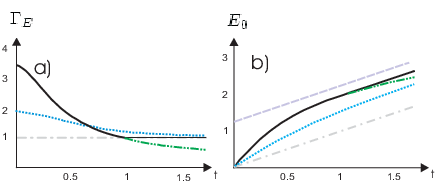
In the Fig. 2 we compare the entanglement rates and the entanglement obtained for different strategies using the “natural Hamiltonian” . As initial state we consider the product of the vacuum state in the first system and the squeezed vacuum in the second system, i.e.,
| (52) |
with squeezing parameter . We compare the strategy in which the rate of entanglement creation is optimized at each time to two simpler ones, namely to just apply the natural Hamiltonian or to simulate the two-mode squeezing Hamiltonian using the optimal scheme of Sec. III. The rate-optimization strategy leads in fact to combination of the other two: one applies first the natural Hamiltonian for a finite time and then (when the “local squeezing” has all been converted to two-mode squeezing) one simulates . Having initially local squeezing available clearly helps with entanglement generation: for an initial unsqueezed state the optimal rate is constant .
Fig. 2b shows that the optimization strategy can lead to noticably more entanglement in the resulting state after finite time: when the entanglement rate is optimized at each point, more entanglement is produced than, e.g., with the interactions or . However, optimizing the rate is in general not the best strategy for the creation of entanglement, see Fig. 3.
IV.2.2 Maximizing the squeezing rate
As in the previous section we are given an interaction Hamiltonian of the form (1), an initial Gaussian state with CM , and we consider the case of infinitesimal interactions. Our goal is here to determine for each and the strategy which maximizes the squeezing rate. We measure squeezing by , where was defined in Eq. (46) as the inverse of the smallest eigenvalue of . The rate we are interested in is
| (53) | |||||
Note that we use the logarithm of instead of for convenience. It simplifies the formulas but since is a monotonic function maximizing the rate of implies a maximal rate for as well ††footnotemark: .
After applying the general strategy to the input state with CM we obtain as in Eq. (44). Doing first order perturbation theory we find that , where is the normalized eigenvector corresponding to the smallest eigenvalue of . We obtain for the squeezing rate:
| (54) |
which is maximized when is as large as possible. Note that
| (55) |
where , where is the –matrix of Eq. (38) and we have used the definitions (37) and (8). One quickly sees that . Writing in its restricted singular value decomposition , where and as in Eq. (26), and using that commute with we see that , where
| (56) |
is the squeezing capability of the Hamiltonian . Note that the matrix is orthogonal with and that we can obtain any such choosing , i.e., by the local operations applied to the initial state. Using the notation , where , we find , which gives an upper bound
for . This maximum can be reached for such that . Given (i.e., ) we can calculate with which satisfies this condition. This then determines the optimal choice of , i.e. how to transform the initial state with CM before letting act in order to maximize the squeezing rate. One simple choice yielding is , i.e. nothing has to be done on the second and . Thus, the optimal input state is given by .
In summary, we have shown that the maximal squeezing rate is given by Eq. (16) as a product of the squeezing capability of the given Hamiltonian and the squeezability of the given state. The optimal CM to let act on is , where
| (57) |
and parallelizes and . Note that the fact that is normalized implies that for any input state. Since we look at the logarithm of the squeezing this implies that .
IV.3 Optimal entanglement generation from the vacuum state
In practice, we are interested in creating the largest amount of entanglement when acts for a finite total time . Optimizing the rate of entanglement creation at each time does lead to a local but not necessarily, as we saw, the global maximum of the entanglement at time Kraus and Cirac 2001.
We now show how to employ the interaction to create the most entanglement in a given time . To this end, we make use of the squeezing of which was introduced in Eq. (46) as the smallest eigenvalue of . The squeezing of is known Wolf et al. 2002 to give an upper bound for the amount of entanglement of , with . We proceed as follows: First we calculate the strongest squeezing that can be achieved after time . This also gives an upper bound for the entanglement that can be obtained during this time. Then we point out a strategy that achieves the optimal squeezing and at the same time the strongest entanglement compatible with the given squeezing, thus being optimal on both counts.
The squeezing capability of a symplectic map , i.e., the factor by which the squeezing in a CM can be increased by the application of , is given by the inverse square of the smallest singular value of , since . Here and in the following we use that for the smallest singular value of a product we have . Now consider the symplectic map corresponding to the unitary evolution generated by an interaction Hamiltonian after time , cf. Eq. (39). The singular values of can easily be calculated analytically. We need them only for small times to first order in , in which case we find:
| (58) |
where are the restricted singular values of the matrix [cf. Eq. (8)] corresponding to .
Since we see immediately that , which implies that the squeezing capability of is bounded by . Now consider a strategy as in Eq. (4), alternating the use of for time with local rotations . Note that the , which sum to , are not assumed to be infinitesimal. The time-evolution effected by this strategy is described by a symplectic map
| (59) |
where and are the local rotations corresponding to . Clearly, . Hence , i.e. we have an upper bound to the amount of squeezing that can be produced from an initially unsqueezed pure state by applying for a total time .
A strategy to achieve this optimum is the following: we choose the local rotations as -rotation in system 1 and in system 2, the times all equal, and consider the limit . This corresponds to the situation considered in Sec. III and simulates the Hamiltonian related to . Let , then we have that , since rotations commute with . That is, apart from local rotations the strategy, which simulates the two-mode squeezing Hamiltonian with an efficiency , which is the optimal factor according to Eq. (29). Letting act for a time (using up an interaction time ) transforms the vacuum state into the two-mode squeezed state with CM
| (60) |
which saturates the bounds derived above, since .
Now we show that in Eq. (60) is also the most entangled state that can be obtained after letting act for a total time . Using Eq. (45) for the negativity of a Gaussian state with CM (i.e. an arbitrary strategy applied to the vacuum state) we get
Since the simulation of two-mode squeezing is the optimal strategy for both squeezing and entanglement generation. Note that even a rough approximation of the optimal strategy, i.e., a strategy consisting of just two or three steps already yields a marked improvement in generated squeezing and entanglement.
Up till now we have only considered the unitary evolution of the initial state. There are, however, further tools available in current experiments. There might be additional light modes (ancillas) in the vacuum state on which passive linear optical operations (described by orthogonal and symplectic transformations) as well as complete or partial homodyne measurements can be performed. In principle these might help to increase the entanglement in , but in the following we show that this is not the case. We consider the following general set-up: consider system with CM , ancilla systems in vacuum state i.e., , linear passive interactions (described by a symplectic and orthogonal matrix ) between the system light mode and the ancillas (e.g. beam splitter between light and ancillary modes), such that the whole system is described by the CM ; clearly, and now we show that a Gaussian measurement does not increase : We write as
where the block matrix refers to the ancillary modes to be measured. Then the resulting state is described by the CM Giedke and Cirac 2002. Using the following characterization of the smallest eigenvalues Horn and Johnson 1987 it is straight forward to see that measurement has reduced the squeezing of the state:
Consequently, unsqueezed ancilla systems and Gaussian measurements are of no help in increasing the squeezing or entanglement in a Gaussian state.
The preceding discussion does not completely solve the problem of optimal entanglement generation with a Hamiltonian , since only one particular initial state (the vacuum) has been considered. If, e.g., the initial state of the light field is squeezed, we have seen in Sec. IV.2 that better rates can be achieved (see Fig. 2), which will translate into larger entanglement after finite times. The methods used above easily yield an upper bound for the entanglement that can be obtained from initially squeezed states: Consider an initial product state with squeezing and in systems 1 and 2 and let . By the same arguments as above, after has acted for a time the squeezing in the final state and the negativity are bounded by . We can find a better bound on the achievable entanglement drawing on results from Ref. Wolf et al. 2002, where it was shown that the negativity of a two-mode CM is bounded by , where are the two smallest eigenvalues of the . This implies that
| (61) |
which yields the dash-dotted curve in Fig. 2b. This bound is most probably not tight for , not even as .
One might think that in order to optimize the entanglement after some finite time it always suffices to optimize the rate at each time as for the case of a vacuum input. For qubit systems this was indeed shown to be true Dür et al. 2001. In contrast, it does not hold for cv systems as the counterexample depicted in Fig. 3 shows: We start with a slightly entangled state with CM which can be obtained from the two-mode squeezed state squeezing both and by . Then the “local squeezing parameter” is zero and the optimal rate therefore . If is small and large it is possible to sacrifice some entanglement in order to “activate” the local squeezing thus enhancing the rate later on and obtaining significantly more entanglement at time .

The difference to the qubit case is related to the fact that in the cv context not all local transformations are available and hence not all equally entangled states are locally equivalent.
V Discussion and Conclusion
We have investigated how a quadratic interaction between two continuous variable systems (as it occurs naturally in certain quantum optical systems) can be optimally used to perform several quantum information tasks when certain simple local control operations (phase space rotations) can be implemented as well. First we have given necessary and sufficient conditions for the simulation of a Hamiltonian evolution given a fixed interaction and fast local rotations. In particular, we have shown that the naturally occurring Hamiltonian Eq. (3) allows to simulate all bilinear Hamiltonians and is in fact of the most versatile kind for this purpose. Moreover we have seen that almost all the Hamiltonians of the form (1) (and in particular ) allow to generate all symplectic transformations on two modes, i.e., the complete group can be generated starting from no more than the three Hamiltonians .
With these results we have addressed the questions of optimal creation of entanglement and squeezing for a two–mode Gaussian state using a given interaction of the form (1) and local rotations of the form , both of which are available in current experiments. For the case of small (infinitesimal) interaction times, we have determined the optimal strategy to increase entanglement or squeezing for any input state, i.e, we have derived the maximal entanglement and squeezing rates and determined the strategies which lead to these maxima. For the general case (finite interaction time) we have derived the optimal strategy for the creation of entanglement and squeezing starting with the vacuum state. We have also shown that (in contrast to qubit systems) for continuous variables optimizing the entanglement rate is not necessarily the best way to generate a finite amount of entanglement.
There are several interesting applications of our results for quantum information processing. In particular, we have seen that the beam splitter Hamiltonian can be simulated with an efficiency factor by . When acting for a time the Hamiltonian generates the swap operation between the systems 1 and 2, thus performing the “write-in” and “read-out” operations needed when the atomic ensemble is to be used as a quantum memory for the state of the light mode Kozekhin et al. 2000.
Another interesting application for atomic ensembles is enabled by the so-called spin-squeezed states Kitagawa and Ueda 1993 which have been prepared experimentally in settings similar to the one described in this paper Hald et al. 1999; Kuzmich et al. 2000. It has been shown that these states allow for a significant increase in the precision of atomic clocks Sørensen et al. 2001. While the methods presented above show efficient ways to create squeezed atomic states (e.g., by using the interaction to create squeezing or entanglement optimally and then project the atoms into a pure squeezed state by measuring the light), it would also be interesting to find the optimal such procedure.
Note that the argument in Sec. IV.3 is easily adapted to similar circumstances. E.g., it was shown in Sørensen et al. 2001 that the interaction between the atoms of a suitably prepared Bose-Einstein–condensate (BEC) can be described by the quadratic Hamiltonian , which can be used to drive the BEC into a spin squeezed state. By the same reasoning as in Sec. IV.3 we see that after an interaction time a squeezing of is the maximum achievable. This shows optimality of the procedure suggested in Sørensen et al. 2001 (which employs effectively the so-called “two-axes counter-twisting” Hamiltonian).
In summary, we have investigated the capabilities of cv interaction Hamiltonians . We have shown which other Hamiltonians can be simulated with such an and the available control operations and how to do so efficiently. Then we have derived the optimal entanglement generation rates achievable with this Hamiltonian and given an optimal protocol for the generation of entanglement between the two modes for finite times.
Acknowledgements.
We acknowledge stimulating discussions with Eugene Polzik. This work was supported in part by the European Union under the project EQUIP (contract IST-1999-11053).Appendix A Proof of the necessary and sufficient condition for Hamiltonian simulation
First we prove necessity. If can simulate efficiently (18) has to hold for and . Therefore and because of (8) and (25) there must exist a probability distribution and special orthogonal matrices such that
| (62) |
Rotation matrices which should in principle appear on the left hand side can be removed by left and right multiplication with corresponding transposed matrices. In (62) we assume these ones to be already included in the on the right hand side.
By using the fact that the vector of the diagonal elements of a product can be written as where denotes the component-wise (so-called Hadamard) product of matrices we can express the last equation in compact form as
| (63) |
The definition of the matrix in (63) is obvious. Using that all matrices are elements of it can be seen easily that
Conditions (28) follow now directly from (63) and these properties of :
The same holds identically for all plus signs replaced by minus signs proving necessity.
To demonstrate sufficiency we show that conditions (28) guarantee the existence of a matrix as in (63) which in turn admits to connect the primed and unprimed restricted singular values as in (62). This provides an efficient simulation protocol of the form (9).
Given and fulfilling (28) we can for the time being assume that and define
With this definition we have . Next we have to show that can be written as a convex sum of Hadamard products of rotation matrices which is in fact exactly what inequalities (28) ensure.
It is again easy to check that if we can find probabilities such that and and therefore
| (64) |
This decomposition of allows to pass from (63) to (62) conserving the diagonal structure as can be checked easily. Thus it suffices to show how (28) implies . Multiplying the first [second] line of (28) by yields respectively
The first term on the right hand sides is nonnegative due to premise (27) such that these inequalities are equivalent to
which is, regarding the definition of and , exactly what we had to show and proves sufficiency for the case .
The complementary cases turn out to be trivial, since conditions (28) then require or respectively and this means that we can exclusively simulate Hamiltonians where . for some local rotations , i.e. has to be - in this sense - locally equivalent to . Hence, nothing has to be shown in this case.
We point out that this proof provides the possibility to construct simulation protocols explicitly. Given and one has to calculate the decomposition in 64. Then the probabilities and rotations appearing there will fix the time steps and control operations in (9). As can be seen such a protocol will contain at most three intervals of interaction and control operations being rotations about and .
Appendix B Gate Simulation
To show that any unitary where is quadratic expression in the operators can be decomposed as given in (III.5) we will proceed in three steps:
(i) As shown in Simon et al. 1994; Braunstein 1999 any such can be decomposed into a sequence of one passive transformation, single mode squeezing and another passive transformation. That is to say the symplectic matrix corresponding to the unitary transformation can be decomposed as where are orthogonal, symplectic and, therefore, passive transformations and the diagonal matrix amounts to local squeezing. Note that this is basically a singular value decomposition of .
(ii) Passive transformations contain essentially beam-splitter transformations and local rotations and it is well known from quantum optics that any such transformation on two modes can be decomposed into a sequence of a pair of local rotations, one beam-splitter operation and another pair of local rotations. Thus, a unitary corresponding to a orthogonal symplectic transformation can be decomposed as where is defined in (32).
(iii) What is left to show is how to attain single mode squeezing. For this we split the matrix into two components, and show how each of them can be attained by means of beam-splitters and two-mode squeezing. Let us denote by and the variants of beam splitter and two-mode squeezing operators which are attained from (32) and (33) respectively by locally rotating . Then it can be easily shown that the sequence generates a symplectic transformation and correspondingly .
Collecting things together and ordering all passive components as in (ii), i.e. such that it contains only one application of a beam-splitter operation, decomposition (III.5) follows immediately.
References
- Furusawa et al. (1998) A. Furusawa, J. L. Sørensen, S. L. Braunstein, C. A. Fuchs, H. J. Kimble, and E. S. Polzik, Science 282, 706 (1998).
- Vaidman (1994) L. Vaidman, Phys. Rev. A 49, 1473 (1994).
- Braunstein and Kimble (1998) S. L. Braunstein and H. J. Kimble, Phys. Rev. Lett. 80, 869 (1998).
- Hald et al. (1999) J. Hald, J. L. Sørensen, C. Schori, and E. S. Polzik, Phys. Rev. Lett. 83, 1319 (1999).
- Julsgaard et al. (2000) B. Julsgaard, A. Kozhekin, and E. S. Polzik, Nature 413, 400 (2000).
- Kuzmich et al. (2000) A. Kuzmich, L. Mandel, and N. P. Bigelow, Phys. Rev. Lett. 85, 1594 (2000).
- Kuzmich and Polzik (2000) A. Kuzmich and E. S. Polzik, Phys. Rev. Lett. 85, 5639 (2000).
- Duan et al. (2000a) L.-M. Duan, J. I. Cirac, P. Zoller, and E. S. Polzik, Phys. Rev. Lett. 85, 5643 (2000a), eprint quant-ph/0003111.
- Duan et al. (2000b) L.-M. Duan, G. Giedke, J. Cirac, and P. Zoller, Phys. Rev. Lett. 84, 2722 (2000b), eprint quant-ph/9908056.
- Simon (2000) R. Simon, Phys. Rev. Lett. 84, 2726 (2000), eprint quant-ph/9909044.
- Werner and Wolf (2001) R. F. Werner and M. M. Wolf, Phys. Rev. Lett. 86, 3658 (2001), eprint quant-ph/0009118.
- Giedke et al. (2001a) G. Giedke, B. Kraus, M. Lewenstein, and J. I. Cirac, Phys. Rev. Lett. 87, 167904 (2001a), eprint quant-ph/0104050.
- Giedke et al. (2001b) G. Giedke, B. Kraus, M. Lewenstein, and J. I. Cirac, Phys. Rev. A 64, 052303 (2001b), eprint quant-ph/0103137.
- Giedke et al. (2001c) G. Giedke, L.-M. Duan, P. Zoller, and J. I. Cirac, Quant. Inf. Comp. 1(3), 79 (2001c), eprint quant-ph/0104072.
- Giedke and Cirac (2002) G. Giedke and J. I. Cirac, Phys. Rev. A 66, 032316 (2002), eprint quant-ph/0204085.
- Eisert et al. (2002) J. Eisert, S. Scheel, and M. B. Plenio, Phys. Rev. Lett. 89, 137903 (2002), eprint quant-ph/0204052.
- Fiurášek (2002) J. Fiurášek, Phys. Rev. Lett. 89, 137904 (2002), eprint quant-ph/0204069.
- Thomsen et al. (2002) L. K. Thomsen, S. Mancini, and H. M. Wiseman (2002), eprint quant-ph/0208160.
- Bouchoule and Mølmer (2002) I. Bouchoule and K. Mølmer (2002), eprint quant-ph/0205082.
- Di Lisi and Mølmer (2002) A. Di Lisi and K. Mølmer (2002), eprint quant-ph/0208172.
- Berry and Sanders (2002) D. W. Berry and B. C. Sanders, Phys. Rev. A 66, 012313 (2002).
- Dür et al. (2001) W. Dür, G. Vidal, J. I. Cirac, N. Linden, and S. Popescu, Phys. Rev. Lett. 87, 137901 (2001), eprint quant-ph/0006034.
- Kraus and Cirac (2001) B. Kraus and J. I. Cirac, Phys. Rev. A 63, 062309 (2001), eprint quant-ph/0011050.
- Zanardi et al. (2000) P. Zanardi, C. Zalka, and L. Faoro, Phys. Rev. A 62, 030301(R) (2000), eprint quant-ph/0005031.
- Dodd et al. (2002) J. L. Dodd, M. A. Nielsen, M. J. Bremner, and R. T. Thew, Phys. Rev. A 65, 040301 (2002), eprint quant-ph/0106064.
- Wocjan et al. (2002) P. Wocjan, M. Rötteler, D. Janzing, and T. Beth, J. Quant. Inf. Comp. 2, 133 (2002), eprint quant-ph/0109063.
- Nielsen et al. (2001) M. A. Nielsen, M. J. Bremner, J. L. Dodd, A. M. Childs, and C. M. Dawson (2001), eprint quant-ph/0109064.
- Bennett et al. (2002a) C. H. Bennett, A. W. Harrow, D. W. Leung, and J. A. Smolin (2002a), eprint quant-ph/0205057.
- Leifer et al. (2002) M. S. Leifer, L. Henderson, and N. Linden (2002), eprint quant-ph/0205055.
- Vidal and Cirac (2002) G. Vidal and J. I. Cirac, Phys. Rev. A 66, 022315 (2002), eprint quant-ph/0108076.
- Bennett et al. (2002b) C. H. Bennett, J. I. Cirac, M. S. Leifer, D. W. Leung, N. Linden, S. Popescu, and G. Vidal, Phys. Rev. A 66, 012305 (2002b), eprint quant-ph/0107035.
- Vidal et al. (2002) G. Vidal, K. Hammerer, and J. I. Cirac, Phys. Rev. Lett. 88, 237902 (2002), eprint quant-ph/0112168.
- Hammerer et al. (2002) K. Hammerer, G. Vidal, and J. I. Cirac (2002), eprint quant-ph/0205100.
- Wolf et al. (2002) M. M. Wolf, J. Eisert, and M. B. Plenio (2002), eprint quant-ph/0206171.
- Kuzmich et al. (1998) A. Kuzmich, N. P. Bigelow, and L. Mandel, Europhys. Lett. 42, 481 (1998).
- Mølmer (1999) K. Mølmer, Eur. Phys. J. D 5, 301 (1999).
- Polzik (1999) E. S. Polzik, Phys. Rev. A 59, 4202 (1999).
- Schori et al. (2002) C. Schori, B. Julsgaard, J. L. Sørensen, and E. S. Polzik, Phys. Rev. Lett. 89, 057903 (2002).
- Duan et al. (2000c) L.-M. Duan, A. Sørensen, J. I. Cirac, and P. Zoller, Phys. Rev. Lett. 85, 3991 (2000c), eprint quant-ph/0007048.
- Duan et al. (2002) L.-M. Duan, J. I. Cirac, and P. Zoller (2002), eprint quant-ph/0205005.
- Arecchi et al. (1972) F. T. Arecchi, E. Courtens, R. Gilmore, and H. Thomas, Phys. Rev. A 6, 2211 (1972).
- Schnabel et al. (2002) R. Schnabel, W. P. Bowen, N. Treps, T. C. Ralph, H.-A. Bachor, and P. K. Lam (2002), eprint quant-ph/0208103.
- Simon et al. (1994) R. Simon, N. Mukunda, and B. Dutta, Phys. Rev. A 49, 1567 (1994), eprint quant-ph/0204069.
- Lloyd and Braunstein (1999) S. Lloyd and S. L. Braunstein, Phys. Rev. Lett. 82, 1784 (1999).
- Vidal and Werner (2002) G. Vidal and R. F. Werner, Phys. Rev. A 65, 032314 (2002), eprint quant-ph/0102117.
- Horn and Johnson (1987) R. A. Horn and C. R. Johnson, Matrix Analysis (Cambridge University Press, 1987).
- Kozekhin et al. (2000) A. E. Kozekhin, K. Mølmer, and E. S. Polzik, Phys. Rev. A 62, 033809 (2000), eprint quant-ph/9912014.
- Kitagawa and Ueda (1993) M. Kitagawa and M. Ueda, Phys. Rev. A 47, 5138 (1993).
- Sørensen et al. (2001) A. Sørensen, L.-M. Duan, J. I. Cirac, and P. Zoller, Nature 409, 63 (2001), eprint quant-ph/0006111.
- Braunstein (1999) S. L. Braunstein (1999), eprint quant-ph/9904002.
- Horn and Johnson (1994) R. A. Horn and C. R. Johnson, Topics in Matrix Analysis (Cambridge University Press, 1994).
- van Enk (1999) S. J. van Enk, Phys. Rev. A 60, 5095 (1999).
- Scutaru (1998) H. Scutaru, J. Math. Phys. 39, 6403 (1998), eprint quant-ph/9908061.