Optimal Sizes of Dielectric Microspheres for Cavity QED with Strong CouplingPreprint: Preprint: Final

Motivated by the pioneering work of Braginsky and Ilchenko Braginsky and Ilchenko 1987, some of the highest quality optical resonators to date have been achieved with the whispering gallery modes (WGMs) of quartz microspheres Gorodetsky et al. 1995; Vernooy et al. 1998a. Over the wavelength range $630-850\mathrm{nm}$, quality factors ${Q\approx 8\times 10^{9}}$ have been realized, and cavity finesse $\mathcal{F}=2.3\times 10^{6}$ demonstrated Gorodetsky et al. 1995; Vernooy et al. 1998a. Such high quality factors make the WGMs of small dielectric spheres a natural candidate for use in cavity QED Vernooy and Kimble 1997; Mabuchi and Kimble 1994; Braginsky and Ilchenko 1987; Gorodetsky and Ilchenko 1994; Treussart et al. 1994; Knight et al. 1995; Knight et al. 1996; Jhe and Kim 1995; Chew 1987; Klimov and Letokhov 1996; Klimov et al. 1996; Klitzing et al. 2001; Mazumder et al. 1996; Campillo et al. 1996; Slusher and Mohideen 1996; Matsko et al. 1994; Norris et al. 1997; Fan et al. 1998.

While much of the work regarding quartz microspheres has centered around achieving the ultimate quality factors Gorodetsky et al. 1995; Vernooy et al. 1998a, the quality factor of the resonator is but one of the factors that determines the suitability of the WGMs for investigations of cavity quantum electrodynamics in a regime of strong coupling. In this case, the coherent coupling coefficient, $g$, for a single atom interacting with the cavity mode must be much larger than all other dissipative rates, including the cavity decay rate, $\kappa$, and the rate of atomic spontaneous emission, $\gamma$; namely $g\gg(\kappa,\gamma)$. Note that $2g=\Omega$ gives the Rabi frequency associated with a single quantum of excitation shared by the atom-cavity system Kimble 1994; Kimble 1998. The atom-field interaction can be characterized by two important dimensionless parameters: the saturation photon number, $n_{0}\propto\frac{\gamma^{2}}{g^{2}}$, and the critical atom number, $N_{0}\propto\frac{\kappa\gamma}{g^{2}}$. Since these parameters correspond respectively to the number of photons required to saturate an intracavity atom and the number of atoms required to have an appreciable effect on the intracavity field, strong coupling requires that $(n_{0},N_{0})\ll 1$. Ideally one would hope to minimize both of these parameters in any particular resonator. Unfortunately, within the context of our current understanding of the loss mechanisms of the WGMs Vernooy et al. 1998a, the critical parameters $(n_{0},N_{0})$ cannot be minimized simultaneously in a microsphere.

Motivated by these considerations, in this paper we explore possible limits for the critical parameters $(n_{0},N_{0})$ for the WGMs of quartz microspheres. Following the analysis of Refs. Mabuchi and Kimble 1994; Vernooy and Kimble 1997; Matsko et al. 1994, we study the particular case of a single atom coupled to the external field of a WGM near the sphere’s surface. We show that there are radii that minimize $(n_{0},N_{0})$ individually, and that there is an “optimal” sphere size that minimizes the geometric mean, $\sqrt{n_{0}\times N_{0}}$, of these two cavity-QED parameters and allows both parameters to be near their respective minima. We also report our progress in the fabrication of small microspheres with radii $a\sim 10\mathrm{\mu m}$, and compare our experimental results for $Q$ with those from our theoretical analysis. Finally, we present a detailed comparison for the state of the art and future prospects for achieving strong coupling in cavity QED for both microsphere and Fabry-Perot cavities. Throughout the presentation, we attempt to develop a general formalism that can be applied to diverse systems. However, for definiteness we also present results for a particular system of some interest, namely an individual Cesium atom coupled to the WGMs of quartz microspheres.

Solving for the mode structure of the resonances of a dielectric sphere in vacuum is a classic problem in electricity and magnetism, and the resulting field distributions have been known for some time Stratton 1997. The electric field of the TM, electric type, modes inside and outside a sphere of refractive index $n$ at free-space wavelength $\lambda_{0}$ are respectively,

and,

where $a$ is the radius of the sphere, $k=\frac{2\pi n}{\lambda_{0}}$ is the wave vector inside the sphere, $j_{l}(x)$ is the spherical Bessel function, $h_{l}^{(1)}(x)$ is the spherical Hankel function, $(\widehat{r},\widehat{\theta},\widehat{\phi})$ are unit vectors, and the ^′ refers to differentiation with respect to the argument. Note that the TM modes have a predominantly radial electric field vector.

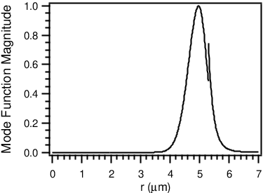
In order to satisfy the boundary conditions at the surface of the microsphere, the tangential components of the mode function immediately inside and outside the sphere must be equal. However, there is a discontinuity in the radial component of the electric field at the dielectric boundary (as can be seen from Fig. 1.) The eigenmodes are determined by solving for the roots of a characteristic equation Stratton 1997, which can be reduced to

Throughout this paper, we normalize the mode functions such that their maximum value is unity. This condition then yields for the $l=m$ modes of the sphere

and,

where

and $N$ is the normalization factor. Because we will require the field outside the sphere to be as large as possible, we will choose the $p=1$ modes. Also, because the coherent coupling constant $g\varpropto\frac{1}{\sqrt{V_{\vec{P}}}}$, where $V_{\vec{P}}$ is the cavity mode volume, we choose the $l=m$ modes, since they yield the smallest electromagnetic mode volume, as will be explained in the next section.

The effective mode volume $V_{\vec{P}}$ associated with the electromagnetic field distribution $\vec{\Psi}(r,\theta,\phi)$ Vernooy and Kimble 1997 is given by

where

and $\vec{P}$ corresponds to the $(p,l,m)$ mode. $V_{Q}$ is the quantization volume discussed in Ref. Vernooy and Kimble 1997. As long as a radius $r_{Q}$ is chosen large enough to include the effects of the evanescent field, the mode volume is relatively insensitive to the particular choice of quantization radius r_q. As discussed more extensively in Refs. Kimble 1994; Kimble 1998 the interaction between the internal atomic degrees of freedom and the intracavity field is characterized by the coherent coupling constant $g(r,\theta,\phi)$, where

and

Note that in the absence of damping, $2g\left(\vec{r}\right)$ gives the frequency for Rabi nutation associated with a single photon in the cavity for an atom initially in the ground state located at position $\vec{r}$ within the mode. Therefore, in order to maximize the coupling strength, one must endeavor to minimize the cavity mode volume.

In order to derive an answer that can be applied to different wavelengths, one can define a dimensionless mode volume parameter, $\tilde{V}$, and plot as a function of a dimensionless sphere size parameter, $\tilde{x}$, defined as:

and

where $V_{\vec{P}}$ is the cavity mode volume, $n$ is the index of refraction at the free-space wavelength $\lambda_{0}$, and $a$ is the sphere radius. The plots then only depend on the index of refraction (see Fig. 2).

Naively, one might assume that the sphere should be made as small as possible in order to minimize the electromagnetic mode volume, and hence to provide a maximum for $g_{0}$ and hence globally for $g\left(\vec{r}\right)$. However, as shown in Figs. 2 and 3, the mode volume for the TM modes of a quartz microsphere actually passes through a minimum at some particular radius $a_{0}$. This behavior can be understood by noting that for $a<a_{0}$, the intrinsic, radiative losses are increasing rapidly and ultimately cause the mode to no longer be well-confined by the sphere, with a concomitant increase of the mode volume. Note that in Fig. 2 and subsequent figures, we give results for $n\sim 1.45$ corresponding to fused silica, as well as for $n=2.00$ and $n=3.00$. These latter cases serve to illuminate the role of $n$ as well as being applicable to other materials (i.e., the index of refraction for GaAs is $n=3.4$ for $\lambda=1550\mathrm{nm}$ Bass 1995). For a very low-OH fused silica microsphere at $\lambda_{0}=852\mathrm{nm}$ (the wavelength of the $D_{2}$ transition in atomic Cesium) with index of refraction $n=1.45246$, the minimum mode volume $V_{\vec{P}}^{\min}\approx 28.4\mu\mathrm{m}^{3}$ occurs for radius $a\approx 3.73\mu\mathrm{m}$ corresponding to mode numbers $p=1,l=m=34$ (see Fig. 3). One might at first believe that this value for the radius represents the optimal sphere size for use as a cavity with single atoms. However, while the mode volume $V_{\vec{P}}$ plays an important role in determining the coupling constant (Eq. 12), it is not the only parameter relevant to cavity QED with single atoms in a regime of strong coupling. As discussed in the next sections, the quality factor, $Q$, of a WGM has a strong dependence on the sphere radius, and must also be considered in an attempt to optimize the critical atom and saturation photon numbers.

For fused silica spheres with radius $a\gtrsim 15\mu\mathrm{m}$, the effect of intrinsic radiative losses can be safely neglected, since they allow quality factor $Q\gtrsim 10^{21}$, as illustrated in Fig. 5. Such large values of $Q$ greatly exceed those imposed by technical constraints of material properties, such as bulk absorption and surface scattering.

However, as one moves to very small spheres with radius $a\lesssim 10\mu\mathrm{m}$, the intrinsic radiative $Q$ falls steeply enough to become the dominant loss mechanism even in the face of other technical imperfections. When assessing the usefulness of microspheres for cavity QED, one must account for the entire set of loss mechanisms to determine the optimal size for the microsphere, which is the subject to which we now turn our attention.

The quality factors of the WGMs of fused silica microspheres are determined by several different loss mechanisms. The overall quality factor can then be calculated by adding the different contributions in the following way Gorodetsky et al. 1995:

where $Q_{\mathrm{rad}}$ is due to purely radiative losses for an ideal dielectric sphere and $Q_{\mathrm{mat}}$ results from non-ideal material properties. The principal mechanisms contributing to $Q_{\mathrm{mat}}$ are scattering losses from residual surface inhomogeneities ($Q_{\mathrm{s.s.}}$), absorption losses due to water on the surface of the sphere ($Q_{\mathrm{w}}$), and bulk absorption in the fused silica ($Q_{\mathrm{bulk}}$). The intrinsic material losses are known very accurately, since they arise from absorption in the material at the wavelength of concern Lin 1991. Considerably greater uncertainty is associated with the losses due to surface scattering and absorption due to adsorbed material on the surface of the sphere, of which water is likely the principal component. We will adopt the models for these losses presented in Refs. Gorodetsky et al. 1995; Vernooy et al. 1998a, extrapolated to the regime of small spheres of interest here.

The ultimate goal that we consider here is to employ the WGMs of quartz microspheres as cavity modes for achieving strong coupling to atoms within the setting of cavity QED. The atom of choice in this paper is Cesium, and in particular, the $D_{2}$ ($F=4\mapsto F^{\prime}=5$) transition in Cesium at $\lambda_{0}=852.359\mathrm{nm}$ as an illustrative example. Such an analysis allows a direct comparison with the state of the art in Fabry-Perot cavities Hood et al. 2001.

The coupling coefficient $g(\vec{r})$ is the coupling frequency of a single atom to a particular cavity mode and corresponds to one-half the single photon Rabi frequency Kimble 1994; Kimble 1998. For an atom located just at the outer surface of the microsphere (i.e., in vacuum) and interacting with a whispering gallery mode $\vec{P}=(p,l,m)$, the coupling coefficient is given by Vernooy and Kimble 1997

where $a$ is the sphere radius, $\frac{\gamma_{\bot}}{2\pi}=2.61\mathrm{MHz}$ is the transverse spontaneous decay rate for our transition in Cesium, $V_{0}=\frac{3c\lambda_{0}^{2}}{4\pi\gamma_{\bot}}$ is the effective volume of the atom for purely radiative interactions, and $V_{\vec{P}}$ is the electromagnetic mode volume of the whispering gallery mode designated by $\vec{P}=(p,l,m)$.

Armed with a knowledge of $g$, we are now able to determine certain dimensionless parameters relevant to the strong coupling regime of cavity QED. In particular, we consider an atom-cavity system to be in the strong coupling regime when the single-photon Rabi frequency, $2g$, for a single intracavity atom dominates the cavity field decay rate, $\kappa$, the atomic dipole decay rate, $\gamma_{\bot}$, and the inverse atomic transit time, $T^{-1}$ Kimble 1994; Kimble 1998. We will defer further discussion of $T^{-1}$, however, this requirement relates to the need for atomic localization Vernooy and Kimble 1997; Mabuchi and Kimble 1994. In the strong coupling regime, important parameters for characterizing the atom-cavity system are the two dimensionless parameters: the saturation photon number, $n_{0}$, and the critical atom number, $N_{0}$. The saturation photon number, given by

corresponds to the number of photons required to saturate an intracavity atom Kimble 1994; Kimble 1998. The critical atom number, defined by

corresponds to the number of atoms required to have an appreciable effect on the intracavity field Kimble 1994; Kimble 1998. Ideally, one hopes to minimize simultaneously both the critical atom number, $N_{0}$, and the saturation photon number, $n_{0}$, which corresponds to simultaneous maxima for both $\frac{g^{2}}{\kappa\gamma_{\bot}}$ and $\frac{g^{2}}{\gamma_{\bot}^{2}}$.

The saturation photon number and critical atom number are useful because of their physical meaning. However, one can define a new dimensionless parameter

that corresponds to the cavity mode volume in units of $\lambda^{3}$ weighted by the inverse of the strength of the mode function at the atomic position. This enables the equations for the saturation photon number and critical atom number to be expressed as:

and

where

and

This parameter, $\beta$, then also determines the coupling coefficient in the following manner:

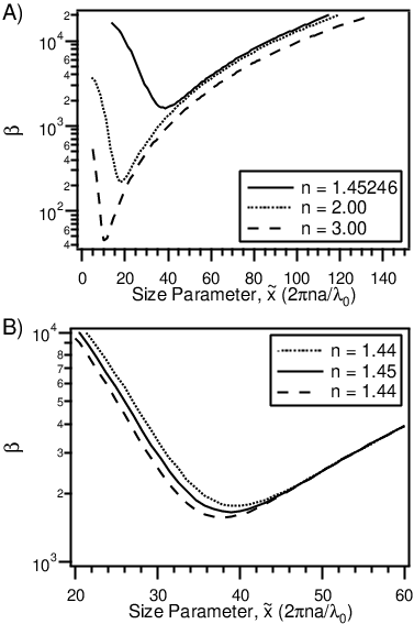
Therefore, we see that one can use a single parameter, $\beta$, combined with the properties of the atom to be used ($\lambda_{0}$ and $\gamma_{\bot}$) and the quality factor of the resonator, $Q_{\mathrm{cavity}}$, to determine the three parameters ($n_{0},N_{0},g_{0}$) of importance in determining the quality of an atom-cavity system.

Figs. 8 and 9 are plots of this dimensionless parameter $\beta$ and of $\frac{1}{\sqrt{\beta}}$ as functions of the dimensionless size parameter $\tilde{x}=\frac{2\pi na}{\lambda_{0}}$ for a few values of index of refraction. Because the index of refraction for fused silica varies from $n=1.444$ at $\lambda_{0}=1550\mathrm{nm}$ to $n=1.458$ for $\lambda_{0}=600\mathrm{nm}$ (see Fig. 4), Figs. 8b and 9b are made for that range of values. From Figs. 8 and 9 one sees that there is a minimum for $\beta$ and a maximum for $\frac{1}{\sqrt{\beta}}$ that depends on the index of refraction.

The results of the previous section can now be used to determine the saturation photon number, $n_{0}$, the critical atom number, $N_{0}$, and the coupling coefficient, $g(a)$, for any atomic transition. In our case, we are concerned with the $D_{2}$ transition in Cesium ($\lambda_{0}=852.359\mathrm{nm}$). For this transition, the spontaneous transverse decay rate is $\frac{\gamma}{2\pi}=2.61\mathrm{MHz}$. Also, at this wavelength the index of refraction for fused silica is $n=1.45246$. This allows one to compute the coupling coefficient, $g(a)=\sqrt{\frac{2\pi c\gamma_{\bot}}{\beta\lambda_{0}}}$. Fig. 10 shows that there is a maximum of $\frac{g}{2\pi}=749.986\mathrm{MHz}$ for a radius $a=3.63\mu\mathrm{m}$, ($l=m=33$). Interestingly, because we are restricted to having the atom couple to the external field of the microsphere, the maximum in the coupling coefficient, $g(a)$, does not coincide with the minimum for the mode volume, $V_{\vec{P}}$ (see Figs. 3 and 10.)

The saturation photon number, $n_{0}$, is proportional to the dimensionless parameter $\beta$ as shown in Eq. 29. Since the factor of proportionality is a constant that depends only on the properties of the particular atom of concern, the curve is determined by that of $\beta$ along with the quality factor of the atomic resonance (in our case Cesium), which is given by Eq. 31 to be $Q_{atom}=6.738\times 10^{7}$. Fig. 11 is a plot of the saturation photon number for the $D_{2}$ transition in Cesium as a function of sphere size. Fig. 11 shows that there is a minimum for the saturation photon number of $n_{0}=6.05527\times 10^{-6}$ for a sphere radius of $a=3.63163\mu\mathrm{m}$ $(l=m=33)$.

The critical atom number, $N_{0}$, is also proportional to the dimensionless parameter $\beta$ as shown in Eq. 30. However, its factor of proportionality is the quality factor of the resonator, $Q_{cavity}$, which has a very strong dependence on the sphere radius, $a$, in the region below 10$\mathrm{\mu m}$ (see Fig. 7). Therefore, the minimum for the critical atom number does not occur for the same sphere size as for the saturation photon number. Fig. 12 is a plot of the critical atom number as a function of sphere size. Using for $Q_{cavity}$ the model that incorporates all of the loss mechanisms discussed in section IV (radiative losses, bulk absorption, surface scattering, and absorption due to water on the surface), we find that the minimum for the critical atom number $N_{0}=8.99935\times 10^{-6}$ occurs for a sphere radius of $a=8.12015\mu\mathrm{m}$ $(l=m=79)$. At this radius, the coupling coefficient is $\frac{g}{2\pi}=304.16\mathrm{MHz}$.

Unfortunately, as illustrated in Fig. 13, the minima for the two parameters, $n_{0}$ and $N_{0}$, do not occur for the same sphere radius. However, if one uses the minimum of the geometric mean of the two parameters, each can have a value near its respective minimum. The minimum of the geometric mean occurs for a sphere radius $a=7.83038\mu\mathrm{m}$ $(l=m=76)$. For this sphere size, the coupling coefficient is $\frac{g}{2\pi}=318.333\mathrm{MHz}$, the saturation photon number is $n_{0}=3.36107\times 10^{-5}$, and the critical atom number is $N_{0}=9.27834\times 10^{-6}$. Therefore, each cavity QED parameter can be made to achieve simultaneously a value near its respective minimum.

A large portion of the work being done on microspheres has been to push the quality factors of the spheres to record levels Gorodetsky et al. 1995; Vernooy et al. 1998a. This effort has produced some of the highest finesse ($\mathcal{F}=2.3\times 10^{6}$) optical cavities to date with quality factors $Q\sim 10^{10}$ Gorodetsky et al. 1995; Vernooy et al. 1998a. However, we have seen that $Q$ is not the only relevant factor in determining the suitability of the WGMs for cavity QED in a regime of strong coupling. In general, the preceding analysis demonstrates the requirement to push to microspheres of small radius, $a\lesssim 10\mathrm{\mu m}$. Unfortunately, the experiments that have achieved the highest quality factors and which have investigated certain material loss mechanisms are of rather larger size, and hence not optimal for cavity QED in a regime of strong coupling. For example, the experiment of Ref. Vernooy et al. 1998a achieved a quality factor of $Q=7.2\times 10^{9}$ at $850\mathrm{nm}$ in a sphere of radius $a=340\mathrm{\mu m}$.

To explore the possibilities of cavity QED with strong coupling in substantially smaller spheres, we have undertaken a program to study fabrication techniques for quartz microspheres with $a\lesssim 30\mathrm{\mu m}$, while still maintaining high quality factors. We have been able to fabricate $10\mathrm{\mu m}$ radius spheres using an oxygen-hydrogen micro-torch to melt the ends of very low-OH fused silica rods to form a sphere on the end of a stem. Light is then coupled to the sphere using frustrated total internal reflection of a prism, as in Refs. Vernooy and Kimble 1997; Vernooy et al. 1998a; Vernooy et al. 1998b. Our observations demonstrate that spheres of this size can be made consistently to have quality factors $Q\gtrsim 0.8\times 10^{7}$. While this is encouraging progress, the resulting $Q$ is two orders of magnitude smaller than the theoretical maximum of approximately $1.3\times 10^{9}$ for this size based upon the model discussed in Section IV.

One possible reason for this discrepancy could be the importance of minimizing the ellipticity of the small spheres. Because the small resonators fabricated by our technique have a stem protruding out of them, they are far from spherical. When coupling to an $l=m$ mode in spheres with $a\gtrsim 100\mathrm{\mu m}$ and hence large $l$, the mode is tightly confined to the equator; therefore, the poles do not have an appreciable impact on the mode structure or quality factor. In this case, it is not of critical importance to have the best sphere possible, but rather the best great circle possible to achieve large quality factors. However, this is not the case in small spheres with $a\lesssim 10\mathrm{\mu m}$. As $a$ decreases, the $l=m$ modes occupy an increasingly larger proportion of the sphere in polar angle, and the ellipticity of the sphere becomes increasingly important in determining the mode structure as well as the $Q$. However, while there is certainly room for improvement in our fabrication technique and in the resulting mode structures and quality factors, we shall see in the next section that the current results have promising implications.

Fig. 14 offers a comparison of the state of the art for Fabry-Perot and microsphere cavities for cavity QED, as well as projections of likely limits for each. It is interesting to note that in our projections for the limiting cases of each, microspheres allow for a significant improvement in the critical atom number, $N_{0}$, relative to Fabry-Perot cavities. On the other hand, a principal advantage of Fabry-Perot cavities relative to microspheres would seem to be significant improvements in the saturation photon number, $n_{0}$. The specific specific task at hand would then dictate which technology to apply.

As shown in Fig. 14, there has already been some progress in coupling atoms to the external fields of a microsphere Vernooy et al. 1998b. The sphere employed for the work of Ref. Vernooy et al. 1998b had a radius of $a\approx 60\mu\mathrm{m}$, and quality factor $Q\lesssim 5\times 10^{7}$, corresponding to a mode volume of $V_{\vec{P}}\approx 3.7\times 10^{3}\mu\mathrm{m}^{3}$, coupling coefficient $g_{a}/(2\pi)\approx 24\mathrm{MHz}$, saturation photon number $n_{0}=5.54\times 10^{-3}$, and critical atom number $N_{0}=2.99\times 10^{-2}$. If instead this experiment were to be implemented with a smaller sphere with $10\mu\mathrm{m}$ radius and with quality factor $Q\sim 0.8\times 10^{7}$ such as we have manufactured and described in Section VI, the following parameters would be achieved: a mode volume of $V_{\vec{P}}\approx 1.4\times 10^{2}\mu\mathrm{m}^{3}$, coupling coefficient $g_{a}/(2\pi)\approx 233\mathrm{MHz}$, saturation photon number $n_{0}\approx 6.27\times 10^{-5}$, and critical atom number $N_{0}\approx 2.11\times 10^{-3}$. Therefore, we see that currently achievable quality factors in spheres of radius $10\mathrm{\mu m}$ already would allow for impressive results in cavity QED with single atoms.

By comparison, the state of the art for Fabry-Perot cavities has already achieved the following results for the $\mathrm{TEM}_{00}$ modes Hood et al. 2000: a cavity finesse of $\mathcal{F}=4.8\times 10^{5}$, a mode volume of $V_{\mathrm{m}}\approx 1.69\times 10^{3}\mu\mathrm{m}^{3}$, coupling coefficient $g_{0}/(2\pi)\approx 110\mathrm{MHz}$, saturation photon number $n_{0}\approx 2.82\times 10^{-4}$, and critical atom number $N_{0}\approx 6.13\times 10^{-3}$. If one then looks at possible limits of Fabry-Perot technology for cavity QED as analyzed in Ref. Hood et al. 2001, the following may be possible; a cavity of length $\lambda_{0}/2$ with a cavity finesse of $\mathcal{F}=7.8\times 10^{6}$ yields coupling coefficient $g_{0}/(2\pi)\approx 770\mathrm{MHz}$, saturation photon number $n_{0}\approx 5.7\times 10^{-6}$, and critical atom number $N_{0}\approx 1.9\times 10^{-4}$.

It is encouraging that the currently achievable results for small sphere manufacture would already allow the WGMs to compete favorably with the current state of the art in Fabry-Perot cavity QED. However, if one were able to manufacture and couple to spheres at the optimal size $a\approx 7.83\mu\mathrm{m}$ with a $Q\sim 9.76\times 10^{8}$ (the theoretical maximum predicted from the analysis of Section IV), the following results could be achieved: a mode volume of $V_{\vec{P}}\approx 90\mu\mathrm{m}^{3}$, coupling coefficient $g_{a}/(2\pi)\approx 318\mathrm{MHz}$, saturation photon number $n_{0}\approx 3.36\times 10^{-5}$, and critical atom number $N_{0}\approx 9.28\times 10^{-6}$. This would represent a significant improvement over the current Fabry-Perot technology and be competitive with the likely limits of Fabry-Perot technology. However, even short of achieving this stated maximum $Q$ for the WGMs, impressive results can already be attained. With a quality factor $Q\sim 0.8\times 10^{7}$ at the optimal sphere radius $a\approx 7.83\mu\mathrm{m}$, one would obtain these same results (i.e., $g_{a}/(2\pi)\approx 318\mathrm{MHz}$ and saturation photon number $n_{0}\approx 3.36\times 10^{-5}$), except that the critical atom number, $N_{0}$, would increase to $N_{0}\approx 1.13\times 10^{-3}$. This is still an impressive gain over the current capabilities of Fabry-Perot cavities for the saturation photon number, with room for improvement in the critical atom number.

Overall, we thus find that the technologies of microspheres and Fabry-Perot resonators each have their advantages and disadvantages. However, there is one notable advantage of microspheres; they can be made cheaply and relatively simply given sufficient training and skill. By contrast, the Fabry-Perot cavities considered here require specialized coating runs with expensive equipment and considerable expertise, which is to be found at only a few locations worldwide. This alone makes microspheres an attractive alternative to Fabry-Perot cavities for cavity QED. Another unique advantage of the WGMs is the ability to control the cavity decay rate, $\kappa$, by controlling the coupling efficiency into and out of the microsphere (e.g., by adjusting the distance between a coupling prism and the microsphere Gorodetsky and Ilchenko 1999.) Furthermore, as one moves to the limit of small cavities, the open geometry of microspheres offers a considerable advantage when compared to the geometry of Fabry-Perot cavities. Such possibilities combined with our projected values of the critical parameters, $(n_{0},N_{0})$, shown in Fig. 14 point to the competitiveness of microspheres with current and future Fabry-Perot technology and demonstrate their potential as a powerful tool for cavity QED in the regime of strong coupling.