Intensity-dependent dispersion under conditions of electromagnetically induced transparency in coherently prepared multi-state atoms.
Abstract
Interest in lossless nonlinearities has focussed on the the dispersive properties of systems under conditions of electromagnetically induced transparency (EIT). We generalize the lambda system by introducing further degenerate states to realize a ‘Chain ’ atom where multiple coupling of the probe field significantly enhances the intensity dependent dispersion without compromising the EIT condition.
pacs
42.50.Gy, 42.50.Hz, 32.80.-t, 42.65.-kThere has been much interest given lately to the enhancement of optical nonlinearities in Electromagnetically Induced Transparency (EIT). Most of the work has focussed on the three-state system in the configuration, which has provided some dramatic examples of nonlinear optical effects. Examples include ultra-slow bib:UltraSlow, stopped bib:StoppedLight and superluminal bib:UltraFast group velocities, coherent sideband generation bib:CoherentSideband etc. All these nonlinear processes depend on the creation of coherent superpositions of the ground states with accompanying loss of absorption, and such mechanisms were described in bib:Nonlinear. Thorough reviews of EIT and its properties can be found in bib:Marangos1998 and bib:MatskoReview2001.
Recent investigations of nonlinear optics at the few or single photon levels have identified four state systems where the probe field simultaneously couples two transitions in the N configuration. Examples of applications for such work include photon blockade bib:PhotonBlockade and two photon absorptive switches bib:AbsorptiveQSwitch. The classical precursors to such experiments have also been performed bib:ATVeebib:deEchaniz2001. Other experiments on the N scheme have been performed by Éntin et al. bib:Entin2000. In order to realize larger nonlinear effects, Zubairy et al. bib:Zubairy2002 suggested an extension where the more usual N configuration was extended to a system with an arbitrary (even) number of states where all the states are resonantly coupled except on the final transition where detuning is present. This scheme shows enhanced nonlinearities of not only but also higher order susceptibilities. One problem with this scheme and the standard N scheme is to do with the need to balance the required nonlinearity and decoherence in the system. To enhance the nonlinearity present in the systems it is important for the detuning of the final probe field to be minimized, however decreasing the detuning increases the amount of the final excited state which is mixed into the coherent superposition state, resulting in an increase in decoherence and optical losses. This problem is to some extent circumvented by the absorptive switch of Harris and Yamomoto bib:AbsorptiveQSwitch by exploiting such losses, and in photon blockade by using the cavity nonlinearity to prevent absorption of the final photon. Still the increase in decoherence proves to be a difficulty in experimental precursors to these processes and causes problems in travelling wave configurations.
An alternative multistate configuration for investigating EIT enhanced nonlinearities is the tripod configuration, studied recently by Paspalakis and Knight bib:Paspalakis2002 and earlier considered by Morris and Shore bib:Morris1983. This system has many of the advantages of the N system, but by maintaining superposition states of the three ground states also avoids the excess decoherence of the N system. Morris and Shore bib:Morris1983 also mentioned a multi-leg extension of the tripod scheme.
Here we present an alternative extension to the standard configuration which we term as the Chain configuration, depicted in Fig. 1. We start with a atom [Fig. 1(a)] with ground states and and excited state . The transition is excited by a probe (coupling) field of frequency and detuning . The probe (coupling) Rabi frequency is . We assume for convenience that the transition frequencies and are equal and that appropriate selection rules ensure that the probe and coupling fields only interact with their designated states (a concrete example of how this can be achieved is described below).

The five-state Chain is an M system and is illustrated in Fig. 1(b). Here the ground states are labelled , , , and the excited states , . The probe field excites the and transitions simultaneously with Rabi frequencies and respectively (different labels are applied to take account of the different coupling strengths of the transitions), whilst the coupling field excites the and transitions with Rabi frequencies and . We note that a complementary work by Matsko et al. bib:MatskoPreprint2002, which looks at Faraday rotation and Kerr nonlinearities in the , N and M schemes, has been performed which confirms some of our predictions about nonlinearities in these systems. An early study of the M scheme in the context of degenerate two level systems was also performed by Morris and Shore bib:Morris1983
The Chain Lambda atom with states is shown in Fig. 1(c). The ground states are denoted , …, , and the excited states , …, . The probe field excites the transition with Rabi frequency and the coupling field excites the transition with Rabi frequency .
In order to gain insight into the problem we consider first the Hamiltonian for the Chain atom with states. Using the rotating wave approximation this can be written
We ignore the decay from the excited states in our analytical analysis in order to gain simple expressions for the dressed states of the field-atoms system and thus gain a clearer understanding of the problem. Furthermore we shall concentrate our analysis on the optical nonlinearities which are present in the vicinity of the dark state, which are relatively insensitive to decay. This is evident by direct comparisons between numerical solutions of the complete master equation with decay, and our decay-free analytic expressions. The Hamiltonian can be conveniently expressed as a tridiagonal matrix with state ordering , , , …, ,
where we have introduced .
Following the approach taken by Kuang et al. bib:Kuangpreprint and Zubairy et al. bib:Zubairy2002, we first calculate the eigenvectors of the Hamiltonian. These can be written as
where varies from to . It is clearly not possible to give general solutions for the ’s for atoms with more than 3 states, although one may simply derive numerical results. However, if we invoke the adiabatic hypothesis bib:Kuangpreprint and assume that the probe detuning is small , the probe field is turned on slowly, and the coupling field resonant, then we may assume that the system evolves solely into the dressed state with energy closest to 0. For convenience we denote this state where is the number of states in the Chain atom. Using MAPLE bib:Maple, and the simplification that , we have derived expressions for . These are presented in table 1 as unnormalized quantities and where . Note that the results for are equivalent to those which appear in Ref. bib:Kuangpreprint and were also used in Ref. bib:deEchaniz2001.
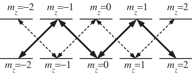
Short of directly creating an artificial atomic structure in a quantum well type material, or in an optical lattice, it is important to investigate whether the required Chain structure is naturally present in any materials. A simple approximate realization to the Chain configuration is obtained by exciting an to transition in an atomic vapor where, as before, is the number of states in the Chain . We illustrate this for the five-state Chain atom in Fig. 2, although the scheme generalizes in an obvious manner. We assume that the coupling field is polarized (and therefore excites transitions from to ) and the probe polarized (exciting transitions from to ). Notice that without any preparation there are two systems here, first the required M system (bold lines in Fig. 2), and second an undesired W system (dashed lines). In order to select the M over the W we first apply the coupling field, this has the effect of optically pumping the population into the state. Next the probe beam is turned on sufficiently slowly to ensure that the system evolves adiabatically to the desired dark state. We also note that the W system does not have any dark states. So even without the adiabatic state preparation, any population in the W system will eventually be optically pumped into the desired dark state of the M system. We also note that the presence of M systems have been identified in conjunction with systems at least twice before in Refs. bib:Morris1983 bib:MatskoPreprint2002. It is important to notice that our method of realizing Chain systems and performing experiments with them, is not significantly more complex than standard experiments on simple systems, all that is necessary to achieve the enhanced nonlinearities is the appropriate choice of transition.
To study intensity-dependent dispersion it is necessary to extract the susceptibility at the probe frequency as a function of small probe detuning
where , being the atomic density and the dipole moment of the transition. The denotes complex conjugation. In order to calculate realistic values of the dispersion which would be attainable in standard experiments with alkali atoms (for example in a magneto-optical trap or vapor cell), we have taken , and .
In order to derive simple results for the nonlinear dispersions, we shall assume the coupling constants for all transitions to be equal, i.e. and so the probe (coupling) field Rabi frequencies are the same for all transitions (). Using MAPLE we can then derive expressions for the intensity dependent dispersion, , for Chain atoms of varying number of states:
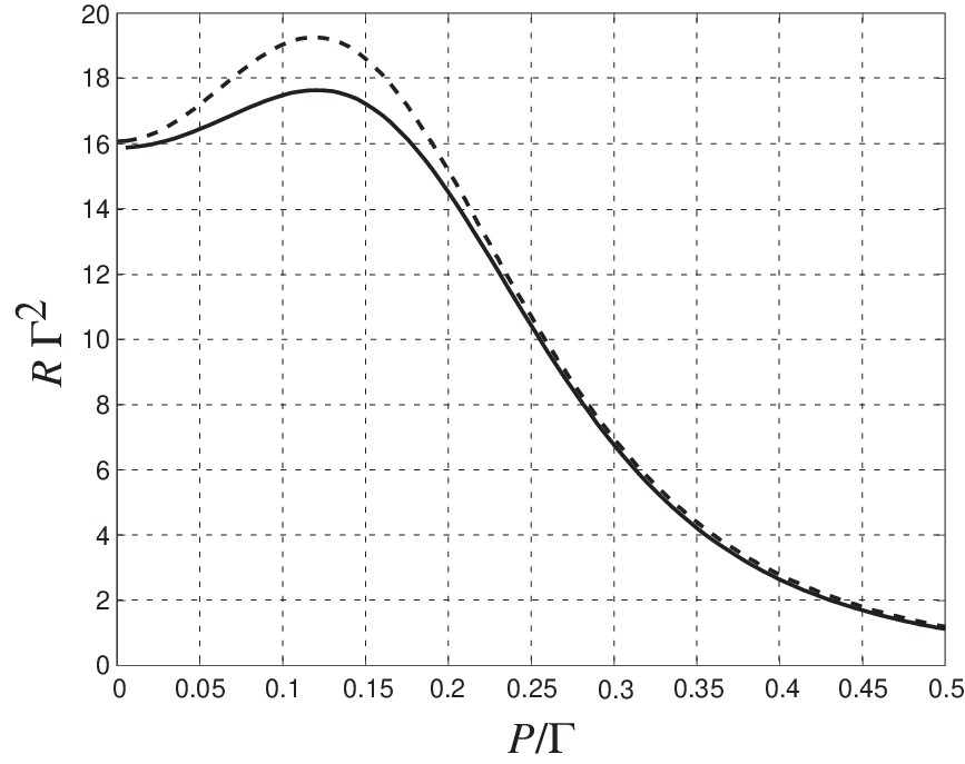
We note that our results for are compatible with the intensity dependent group velocities derived in Ref. bib:Kuangpreprint. The analytically determined dispersions are plotted in Fig. 3 as a function of for . In Fig. 4 we present a comparison between the analytical results for the intensity dependent dispersion and that obtained by solving the density matrix equation with decay given in the Appendix. The good agreement shows that our analytic approach is justified.
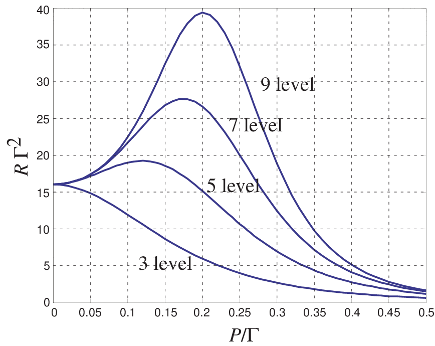
If one simply performs a Taylor series expansion on our results for the ’s (which are non-perturbative), it is easy to show that the Chain systems exhibit nonlinearities to all orders in . The linear dispersion has previously been identified as being important in EIT systems (see for example Harris et al. bib:HarrisPRA1992), and it is clear from Fig. 3 that the linear dispersion is identical for all Chain atoms. From this we may conclude that in the limit of weak probe fields, the probe field cannot couple the levels in any fashion other than the simple scheme. However as the probe intensity is increased, higher-order process begin to turn on. In order to rigorously determine the order of the nonlinearities present, one should construct an effective Hamiltonian, following methods presented by, for example, Zubairy et al. bib:Zubairy2002 or Klimov et al. bib:KlimovQuantPh2002. This has not yet been performed for the Chain system and it is hoped that such investigations will shed more light on the nonlinear optical properties of these systems.
An interesting feature to note in the dispersion calculations is the Rabi frequency ratio which provides the maximum dispersion. In this simple case, the position of the maximum depends only upon the ratio . If is the value of this ratio at the maximum then for the dispersion will be monotonically increasing with increasing , and for it monotonically decreases. It is clear that reciprocal results will be obtained for the corresponding group velocities. For , , and state atoms, the values of are and (to 3 significant figures) respectively.
One material property dependent on the dispersion is the group velocity, which is
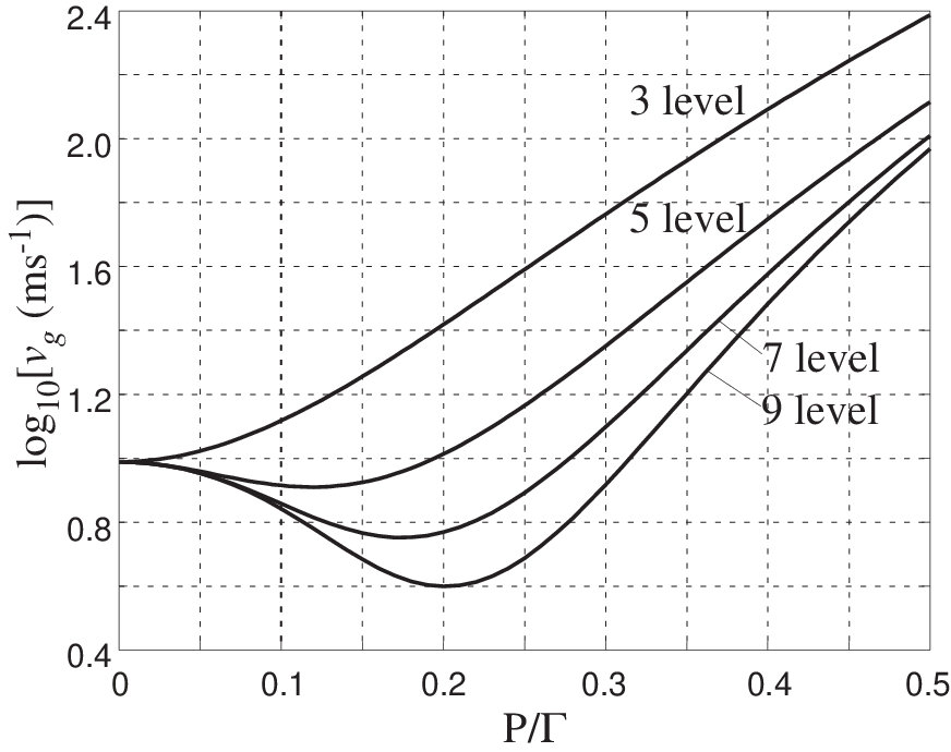
where is the complex refractive index. It is important to realize that in systems with nonlinear dispersions as large as those for Chain systems, the group velocity may be a poor parameter. This is because for realistic propagation through an optically thick medium, the intensity dependence of the medium will alter the shape of a simple gaussian pulse. There are however, other experiments sensitive to the group velocity which may be considered, for example bichromatic excitation of the probe beam to generate a beat note bib:MatskoReview2001 or the use of a frequency modulated (rather than the more usual amplitude modulated) probe signal. In Fig. 5 we present intensity dependent group velocities for , , and state Chain atoms corresponding to the dispersion calculations presented in Fig. 3.
The analytical results given above cannot provide a complete description of the physically realizable problem, because of the different Clebsch-Gordan coupling between the states involved in the transitions. If we use the scheme suggested in Fig. 2 for the couplings and define our coupling strengths relative to the coupling in the first system (i.e. ) then we may write down the expressions for the other couplings in terms of these quantities bib:CGCalc. These are summarized in table 2 for the 5 and 7 state Chain atoms, and it is easy to generalize to higher orders.
| 5-state | 7-state | |
|---|---|---|
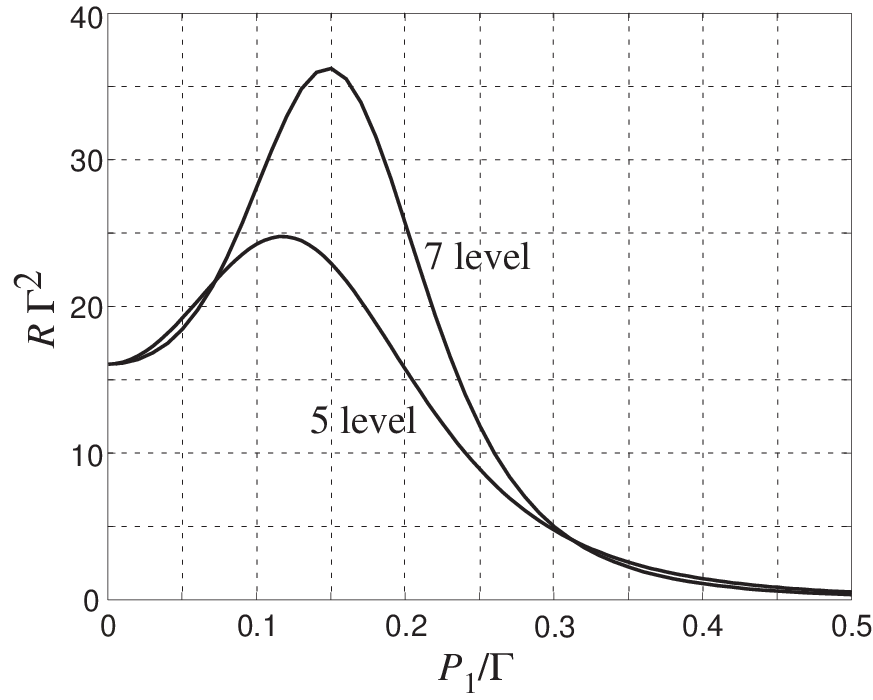
Results of numerical calculations of intensity-dependent dispersions for 5- and 7-state Chain systems are presented in Fig. 6. Comparing Figs. 3 and 6, shows that despite the differences in the values obtained for the dispersions, there is only minimal change to the overall shape of the intensity dependent curves.
We have shown that there exist interesting nonlinear properties for Chain atoms, and in particular we have focussed on the intensity-dependent dispersion as a measure for these nonlinear optical properties. The nonlinearity of these systems increases as the number of atomic states increases, whilst the EIT transparency is maintained. It therefore appears likely that such multistate systems will be useful in the search for new quantum non-linear optical materials. Our analysis has been confined to the optically thin regime. Clearly, in a full study, which would include intensity-dependent group velocities in such highly nonlinear media, it is important to understand propagation effects and especially the effect of such high nonlinearities on pulse shape. Such analysis goes beyond our simple picture and will be the focus of future work.
I Acknowledgements
One of the authors (AG) would like to acknowledge useful discussions with Dr A.B. Matsko (Jet Propulsion Laboratory) and financial support from the EPSRC (UK).
II Appendix
In this appendix we present the density matrix equations of motion for the 5-state Chain atom (M scheme). The equations to be solved are:
For reasons of space we split the Hamiltonian superoperator into smaller sub-blocks, thus
where , and . is the identity matrix and
where . The loss operator is
where the off-diagonal blocks have all elements zero except the which is . The ’s are all diagonal matrices, with non-zero elements
where is the photon dephasing and is the total decay rate from either excited state.
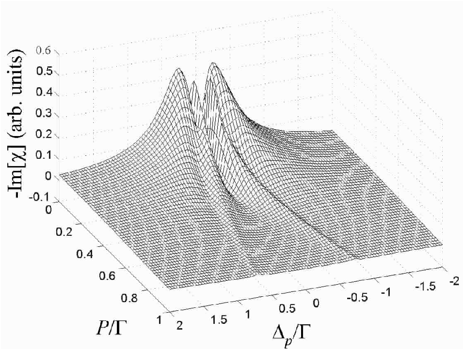
A three-dimensional plot showing as a function of probe detuning, and probe Rabi frequency, for , , and other parameters as above, for the five-state Chain system is presented in Fig. 7.
References
- (1) M. M. Kash, V. A. Sautenkov, A. S. Zibrov, L. Hollberg, G. R. Welch, M. D. Lukin, Y. Rostovtsev, E. S. Fry, and M. O. Scully, Phys. Rev. Lett. 82, 5229-5231 (1999); L. V. Hau, S. E. Harris, Z. Dutton, and C. H. Behroozi, Nature (London) 397, 594-8, (1999); J. P. Marangos, ibid. 397, 559-560 (1999).
- (2) O. Kocharovskaya, Y. Rostovtsev, and M. O. Scully, Phys. Rev. Lett. 86, 628 (2001); C. Liu, Z. Dutton, C. H. Behroozi, and L. V. Hau, Nature (London) 409, 490 (2001); D. F. Phillips, A. Fleischhauer, A. Mair, R. L. Walsworth, and M. D. Lukin, Phys. Rev. Lett. 86, 783 (2001); A. V. Turukhin, V. S. Sudarshanam, M. S. Shahriar, J. A. Musser, B. S. Ham, and P. R. Hemmer, ibid. 88, 023602, (2002).
- (3) A. M. Steinberg and R. Y. Chiao, Phys. Rev. A 49, 2071 (1994); L. J. Wang, A. Kuzmich, and A. Dogariu, Nature (London) 406, 277 (2000); A. Dogariu, A. Kuzmich, and L. J. Wang, Phys. Rev. A 63, 053806 (2001).
- (4) H. Schmidt and R. J. Ram, Appl. Phys. Lett. 76, 3173 (2000), A. F. Huss, N. Peer, R. Lammeggar, E. A. Korsunsky, and L. Windholz, Phys. Rev. A 63, 013802 (2001).
- (5) S. E. Harris, J. E. Field, and A. Imamoğlu, Phys. Rev. Lett. 64, 1107 (1990).
- (6) E. Arimondo, Progress in Optics (Amsterdam: Elsevier 1996) Vol. XXXV, edited by E. Wolf, p. 257; J.P. Marangos, J. Mod. Opt. 45, 471-503 (1998).
- (7) A. B. Matsko, O. Kocharovskaya, Y. Rostovtsev, G. R. Welch, A. S. Zibrov, and M. O. Scully, Adv. At. Mol. Opt. Phys. 46, 191 (2001).
- (8) A. Imamoglu, H. Schmidt, G. Woods, and M. Deutsch, Phys. Rev. Lett., 79, 1467 (1997); S. Rebić, S. M. Tan, A. S. Parkins, and D. F. Walls, J. Opt. B: Quantum Semiclass. Opt. 1, 490 (1999); K. M. Gheri, W. Alge, and P. Grangier, Phys. Rev. A 60, R2673 (1999); A. D. Greentree, J. A. Vaccaro, S. R. de Echaniz, A. V. Durrant and J. P. Marangos, J.Opt. B: Quantum Semiclass. Opt. 2, 252-259 (2000); S. Rebić, A. S. Parkins, and S. M. Tan, Phys. Rev. A 65, 043806 (2002); S. Rebić, A. S. Parkins, and S. M. Tan, ibid. 65, 063804 (2002).
- (9) S. E. Harris and Y. Yamamoto, Phys. Rev. Lett. 81, 3611 (1998).
- (10) M. Yan, E. G. Rickey, and Y. Zhu, Opt. Lett. 26, 548 (2001); M. Yan, E. G. Rickey, and Y. Zhu, Phys. Rev. A 64, 013412 (2001); M. Yan, E. G. Rickey, and Y. Zhu, ibid. 64, 041801 (2001); M. Yan, E. G. Rickey, and Y. Zhu, J. Mod. Opt. 49, 675 (2002).
- (11) S. R. de Echaniz, A. D. Greentree, A. V. Durrant, D. M. Segal, J. P. Marangos, and J. A. Vaccaro, Phys. Rev. A 64, 013812 (2001).
- (12) V. M. Entin, I. I. Ryabtsev, A. E. Boguslavskii, and I. M. Beterov, Pis’ma. Zh. Éksp. Teor. Fiz. 71, 257 (2000) [JETP Lett. 71, 175 (2000)].
- (13) M. S. Zubairy, A. B. Matsko, and M. O. Scully, Phys. Rev. A 65, 043804 (2002).
- (14) E. Paspalakis and P.L. Knight, J. Mod. Opt. 49, 87 (2002).
- (15) J.R. Morris and B.W. Shore, Phys. Rev. A 27, 906 (1983).
- (16) A.B. Matsko, I. Novikova, G.R. Welch, and M.S. Zubairy, Enhancement of Kerr nonlinearity via multi-photon coherence, preprint arXiv:quant-ph/0207141.
- (17) L. Kuang, G. Chen, and Y. Wu, Giant non-linearities accompanying electromagnetically induced transparency, preprint arXiv:quant-ph/0103152 v2 (2001).
- (18) MAPLE 8, Waterloo Maple Inc., 2002.
- (19) S. E. Harris, J. E. Field, and A. Kasapi, Phys. Rev. A 46, R29 (1992).
- (20) A. B. Klimov, L. L. Sánchez-Soto, A. Navarro, and E. C. Yustas, Effective Hamiltonians in quantum optics: a systematic approach, preprint arXiv: quant-ph/0209013 v1 (2002).
- (21) There are many good routines available on the internet. We used one at http://www.ph.surrey.ac.uk/˜phs3ps/cgjava.html to calculate our results.