Spin network quantum simulator

In the past few years there has been a tumultuous activity aimed to proposing novel conceptual schemes of interpretation of quantum computation. Curiously enough, most of them are based on topological notions. Among these, anyonic quantum computation Kit2, fermionic quantum computation Kit1, localized modular functor quantum field computation FrLaWa, holonomic quantum computation ZaRa have mostly attracted attention. Such models appear to be simply different realizations of a unique conceptual scheme that incorporates all of them as particular instances. In this note we aim to claiming that such schemes may all be identified with a model of quantum simulator (in the sense of Feynman Fey) based on (re)coupling theory of $SU(2)$ angular momenta (see, e.g. BiLo and references therein). The paper raises a number of issues without entering in too many technical details but rather trying to establish the guiding philosophy, and is therefore foundational.

The scheme automatically incorporates all the essential features that make quantum information encoding so much more efficient than classical: it is fully discrete (including its time-like variable); it deals with inherently entangled states, and thus incorporates all achievable complexity in its set-up, which is naturally endowed with a tensor product structure; it allows for generic encoding patterns.

In ref.Fey Feynman lists a minimal set of requirements as essential for the proper characterization of an efficient quantum simulator: i) locality of interactions; ii) number of ’computer’ elements proportional to (a function at most polynomial of) the space-time volume of the physical system; iii) time discreteness (time is ’simulated’ in the computer by computational steps). Our argument is based on the fact that all such basic features are typical of spin networks.

By ’spin networks’ we mean here – contrary to what happens in solid state physics, but somewhat in the spirit of combinatorial approach to space-time representation Pen – graphs the node and edge sets of which can be labelled by quantum numbers associated with $SU(2)$ irreducible representations and by $SU(2)$ recoupling coefficients, respectively. Spin networks can thus be thought of as an ideal candidate conceptual framework for dealing with tensorial transformations and topological effects in groups of observables. The idea is to exploit to their full extent the discreteness hypotheses ii) and iii), by modelling the computational space in terms of a set of combinatorial and topological rules that mimic space-time features in a way that automatically includes quantum mechanics.

We begin by defining the structural setting of a universal quantum simulator ${\mathfrak{M}}$ which satisfies all axioms proper to the quantum Turing Machine Man. ${\mathfrak{M}}$, whose computational space is identified with a spin network, can encode information, undergo unitary transformations, and simulate any finite quantum system completely described by eigenstates of $SU(2)$ angular momentum operators. In the sequel we shall indicate how such a scheme can be extended to mixed states.

The machine ${\mathfrak{M}}$ building blocks are an ordered collection of $n+1$ mutually commuting angular momentum operators $\{{\bf J}_{\ell}\,|\,\ell=1,\dots,n+1\}$ (for example associated with a set of $n+1$ kinematically independent particles), with eigenvalues parametrized by $j_{1},\dots,j_{n+1}$, with $j_{\ell}=0,\frac{1}{2},1,\frac{3}{2},\dots$. Such operators are assumed to sum to a sharp total angular momentum ${\bf J}$ with projection $J_{z}$, whose quantum numbers are, respectively, $j$ and $m$, $-j\leq m\leq j$ in integer steps.

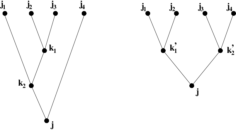
For any given pair $(n,j)$, all possible binary coupling schemes of the $n+1$ angular momenta $j_{\ell}$ together with the the quantum numbers $k_{1},\dots,k_{n-1}$ corresponding to the $n-1$ intermediate angular momenta, provide the ’alphabet’ in which quantum information is encoded. The resulting Hilbert spaces ${\cal H}^{j}_{n}(k_{1},\dots,k_{n-1})$, each $(2j+1)$-dimensional, are spanned by complete orthonormal sets of the form

Such states can be pictorially represented by rooted labelled binary trees in which each node corresponds to an angular momentum quantum number: the root of the tree to $j$, the internal nodes to the intermediate $k_{1},\dots,k_{n-1}$, and the terminal nodes to $j_{1},\dots,j_{n+1}$. An equivalent representation is the binary bracketings notation proposed in BiLo. Fig.1 shows an example of these kinds of representation where, fixed an ordering $j_{1},j_{2},\ldots,j_{n+1}$ and given a common $j$, there exists a correspondence between states given in (1) and the (equivalent) combinatorial structures represented by binary bracketings and labelled binary trees (cfr. e.g. Sta).

Fig. 1

Notice moreover that to each of these assignments (states (1)), there corresponds a unique non-associative structure over the tensor product ${\cal H}^{j_{1}}\otimes\cdots\otimes{\cal H}^{j_{n+1}}\equiv{\rm span}\{|j_{1}m_{1}\rangle\otimes\cdots\otimes|j_{n+1}m_{n+1}\rangle\}$, which is manifestly intrinsically entangled.

A code, in this picture, is a sort of generalized quantum Gödel number in the base associated with a field made of the ordered labels of the intermediate angular momenta, which range over a finite domain (e.g. for ${\bf J}_{1}+{\bf J}_{2}={\bf J}_{12}$, $|j_{1}-j_{2}|\leq j_{12}\leq j_{1}+j_{2}$), as well as the coupling brackets. Such coding spans (and defines) the space of all possible computational states.

In the structure described above, any quantum operation is implemented by some transformation connecting pairs of binary coupled states, namely by the so called ’recoupling coefficients’, or $3nj$ symbols VaMoKh, BiLo.

Indeed the $3nj$ symbols are unitary probability amplitudes

$|{\cal U}_{3nj}|^{2}$ representing the probability that the system, once prepared in state $|j_{1},\dots,j_{n+1};k_{1},\dots,k_{n-1};j,m\rangle$, is measured in state $|j_{1},\dots,j_{n+1};\,k^{\prime}_{1},\dots,k^{\prime}_{n-1};j,m\rangle$.

Notice that the recoupling coefficients can be interpreted as reduced matrix elements since the total magnetic quantum number $m$ can be neglected in view of the Wigner-Eckart theorem. Since they give the elements of the transfer matrices connecting any pair of states, the symbols actually provide the (matrix) analog of the transition function of the quantum Turing Machine Man.

Moreover as any transfer from a state to another – states being in one-to-one correspondence with the vertices of a suitable graph ${\mathfrak{G}}_{n}$ as we shall see below – can be thought of as a (discrete) path integral, $3nj$ symbols implicitly define an ’action’ (and hence an associated hamiltonian operator).

We shall show in the next section that programming ${\mathfrak{M}}$ consists just in selecting which transformations do perform the desired computation.

The computational space associated with ${\mathfrak{M}}$ is a graph ${\mathfrak{G}}_{n}$ whose vertices are identified (i.e. are in one-to-one correspondence) with the system pure angular momentum eigenstates defined in (1).

The Racah transform ${\cal R}$, together with the phase transform $\Phi$,

exhaust all possible transformations between pairs of binary coupling schemes for any $n$. We shall refer to this statement as Biedenharn-Louck theorem (topic 12 in BiLo). Interpreted as transformations on binary trees, ${\cal R}$ and $\Phi$, represented pictorially in Fig.2 and Fig.3, are referred to as rotations and twists, respectively.

The coding proposed above requires both types of operations, (2) and (3), and the corresponding graph is the full twist–rotation graph ${\mathfrak{G}}_{n}$, the vertices of which are to be associated with the computational states of the Machine and the bonds with either Racah or phase transforms. However, in what follows, in order to make exemplification simpler we shall limit our attention to rotation graphs only, i.e. ${\mathfrak{G}}_{n}$-graphs in which adjacent vertices differing only for a twist are identified, since they actually capture all the essential mathematical properties of our model. Fig.4 exhibits for the case $n=3$ the local reduction of ${\mathfrak{G}}_{3}$ when such identification is implemented (cfr. AqCo).

Fig. 4

Accordingly, the bonds of the rotation graph (that we still denote ${\mathfrak{G}}_{n}$) correspond to Racah transforms, possibly apart from weight/phase factors. Fig.5 shows an example of such reduced computational space for $n=3$.

Fig. 5

The combinatorial structure of ${\mathfrak{G}}_{n}$ is fully determined by the identities connecting $6j$ symbols VaMoKh:

i) the Biedenharn-Elliot identity generates pentagon plaquettes in ${\mathfrak{G}}_{n}$:

$$\sum_{x}(-)^{R+x}(2x+1)\left\{{{a\,b\,x}\atop{c\,d\,p}}\right\}\left\{{{c\,d\,x}\atop{e\,f\,q}}\right\}\left\{{{e\,f\,x}\atop{b\,a\,r}}\right\}=\biggl\{{{p\,q\,r}\atop{e\,a\,d}}\biggr\}\left\{{{p\,q\,r}\atop{f\,b\,c}}\right\}\;,$$

ii) Racah’s identities generate triangles:

$$\sum_{x}(-)^{p+q+x}(2x+1)\left\{{{a\,b\,x}\atop{c\,d\,p}}\right\}\left\{{{a\,b\,x}\atop{d\,c\,q}}\right\}=\biggl\{{{a\,c\,q}\atop{b\,d\,p}}\biggr\}\;,$$

here the spin variables $\bigl\{a,b,c,\dots,x\bigr\}$ ranges over all possible values in $\bigl\{0,\frac{1}{2},1,\frac{3}{2},\dots\bigr\}$ which obey the required triangular conditions, and $R=a+b+c+d+e+f+p+q+r$. We argue that the greater computational power of a quantum computer can be ascribed to the feature that its state space ’volume’ grows very rapidly. Indeed the order ($\#$ of vertices) of ${\mathfrak{G}}_{n}$ is $|{\mathfrak{G}}_{n}|=(2n-1)!!$ ($\sim n^{n}$ for large $n$), whereas the diameter ${\mathfrak{d}}_{n}$ of ${\mathfrak{G}}_{n}$ grows approximately as $n\ln n\sim\ln|{\mathfrak{G}}_{n}|$ FaLiVa. In the present scheme ${\mathfrak{d}}_{n}$ is an upper bound for the time-length (number of steps) of the computations machine ${\mathfrak{M}}$ can perform (notice that for the full twist-rotation graph the cardinality is a factor $2^{n}$ larger).

Universality of ${\mathfrak{M}}$, being its computational space ${\mathfrak{G}}_{n}$, is guaranteed by Biedenharn-Louck’s theorem (which plays the role of a sort of generalized Cayley’s theorem): any unitary transformation corresponding to an operation of ${\mathfrak{M}}$ can be reconducted to a finite sequence of operations in ${\mathfrak{G}}_{n}$.

This gives an answer to the question raised by Feynman about universality Fey, explicitly defining the class of ’exact imitators’ of any finite, discrete quantum system, with no need of resorting to the notions coming from the (inherently classical) Boolean circuit theory.

${\mathfrak{M}}$ has all the requisites of the ’quantum simulator’ as defined by Feynman Fey: locality, reflected in the bracketing structure, which bears on the existence of local interactions; discreteness, both of the computational space and of ’time’, and universality. The time lapse from $|in\rangle$ to $|out\rangle$, as required in Feynman’s scheme and as we shall see in the next section, is simulated both through the ordering induced by the graph combinatorial structure and by the number of computational steps; in other words, it is not only discrete but intrinsically inherent to the simulator structure Ll. It is the interplay between such space and time discreteness which gives rise in a natural way to entanglement, due to the clustering proper to the (non associative) Hilbert space tensor product structure generated by the recoupling.

The above ingredients completely define the kinematical structure of ${\mathfrak{M}}$. Further notions are necessary to equip it with the dynamical structure necessary to make it operate.

As in a classical Turing Machine Man, computation is a map from the input data to the output state: ${\cal U}_{\cal P}:|in\rangle\mathrel{\mathop{\longrightarrow}\limits^{{\cal P}}}|out\rangle$, where now the machine states are coded in vectors of the Hilbert spaces ${\cal H}_{n}^{j}$ corresponding to the vertices of ${\mathfrak{G}}_{n}$ and ${\cal U}_{\cal P}$ is the class of unitary tranformations induced by the program ${\cal P}$ and defined by the corresponding $3nj$ symbols.

The structure of computation in ${\mathfrak{M}}$ is a generalization of the conventional Boolean scheme. To begin with, the coding language is based on an ^′alphabet^′ consisting in all the (possibly different) values $j_{\ell}\;,\;\ell=1,\dots,n+1$, of the coupled angular momenta, the intermediate variables $k_{1},\dots,k_{n-1}$, as well as the bracketing structure, and is therefore much more powerful and flexible.

The program ${\cal P}({\mathfrak{A}})$ to perform algorithm ${\mathfrak{A}}$ is the specification of a suitably designed (i.e. depending on ${\mathfrak{A}}$) ordered sequence of ^′local alterations^′ of the alphabet elements in the running state, which play the role of gates. Such alterations are transforms of type (2), possibly accompanied by local permutations of labels and/or subtrees (moves of type (3), phase swaps) in ${\mathfrak{G}}_{n}$. We shall denote any such sequence by $|{\mathfrak{b}}_{\alpha}\rangle$, where index $\alpha$, which keeps track of the given ordering, is such that $|{\mathfrak{b}}_{\alpha+1}\rangle$ is connected to $|{\mathfrak{b}}_{\alpha}\rangle$ by the elementary move corresponding to the local operation required by ${\mathfrak{A}}$, while $|{\mathfrak{b}}_{0}\rangle\equiv|in\rangle$ and $|{\mathfrak{b}}_{L}\rangle\equiv|out\rangle$. $L=L({\cal P}({\mathfrak{A}}))$ is the number of elementary steps required by program ${\cal P}({\mathfrak{A}})$ to complete algorithm ${\mathfrak{A}}$. The associated lexicographically ordered sequence $\{|{\mathfrak{b}}_{\alpha}\rangle\,|\,\alpha=0,\dots,L\}$ defines a directed path in ${\mathfrak{G}}_{n}$ of length $L$ in one-to-one correspondence with the duration of ${\cal P}$ in units of its intrinsic discrete time step $\tau$.

The associated unitary ${\cal U}_{{\cal P}({\mathfrak{A}})}$

where $:\bullet:$ denotes ^′ordered product^′, is a sort of superselection rule which induces destructive interference of the forbidden (i.e. not leading to the correct result) paths in ${\mathfrak{G}}_{n}$. Moreover, each elementary transfer matrix in (4) can be associated with a local hamiltonian operator

It is worth noticing that ^′local^′ is here intended with respect to the computational space ${\mathfrak{G}}_{n}$ of ${\mathfrak{M}}$. When (5) is inserted in (4), hamiltonians $H({\mathfrak{b}}_{\alpha},{\mathfrak{b}}_{\alpha+1})$ generally do not commute with each other and are ^′virtual^′, in the sense that they are generated by the machine dynamics in the course of the computation process. In the physical interpretation, however, they correspond to complex polylocal, many angular momentum binary interactions and simulate even more complex quantum physical systems (e.g., sets of interacting entangled fermions and/or bosons).

Given two generic states $|in\rangle$, $|out\rangle$ in ${\mathfrak{G}}_{n}$, one can consider the Inverse Problem, namely read from the minimum length path the optimal algorithm that computes $|out\rangle$ as result of the application of some ${\cal U}_{{\cal P}({\mathfrak{A}})}$ to $|in\rangle$. The problem of finding the minimum-length path between two given vertices in ${\mathfrak{G}}_{n}$ is a ^′hard^′ combinatorial problem, conjectured to be an NP-c problem (the question however is still open, Pal and references therein): we argue that the spin network simulator ${\mathfrak{M}}$ may support algorithms to solve in polynomial time such kind of problems, because it is known SlTaTh that, at least in the case of unlabelled terminal nodes, the maximum distance between any pair of binary trees with $N$ internal nodes is at most linear in $N$.

The dynamical behaviour of the spin network simulator is closely related to topological quantum field theories Qui. In particular, the sum over all ordered paths in ${\mathfrak{G}}_{n}$ between $|in\rangle$ and $|out\rangle$ of the functionals introduced in (4) has the form of a path-integral for a discrete topological quantum theory in (0+1) space-time dimensions. The topological (combinatorial) invariance is ensured by the equivalence of paths in ${\mathfrak{G}}_{n}$ under the set of identities for the $6j$ symbols discussed in Sect. II. Discretized models based on the recoupling theory of angular momenta have been extensively studied also in 3- and 4-dimensional quantum gravity on the grounds of the seminal paper PoRe (see, e.g. CaMa and references therein).

On the other hand, continuous gravity in (2+1) dimensions is well described by a Chern-Simons-Witten topological quantum field theory, whose basic objects are closed surfaces $\Sigma$ of genus $g$. Freedman et al. in FrLaWa resort just to the latter theory, by considering ’unitary topological modular functors’ $h$, i.e. operations which – assigned a finite dimensional Hilbert space ${\cal H}(\Sigma)$ to any such surface – connect diffeomorphic pairs $\Sigma$, $\Sigma^{\prime}$. To each $h$ there corresponds a transformation ${\cal H}(\Sigma)\longrightarrow{\cal H}(\Sigma^{\prime})$, realized in a quantum algebra. For special choices of this algebra, any such transformation is shown to be in one-to-one correspondence with a product of $\nu$ elementary gate-operations, with ${\cal H}$ interpreted as the computational space of a Quantum Circuit Model. The interger $\nu$, which measures the complexity of the corresponding ’computation’, is linear in the length $\lambda$ of $h$ as a word in the standard generators (Dehn’s twists) of the ’mapping class group’ of $\Sigma$ (whose compositions are cobordisms). Since $\lambda$ is in turn linear in the genus $g$, Freedman concludes that there exists a quantum circuit model that can efficiently simulate any topological modular functor in the given class. On the other hand, as the presentation of a 3-manifold by surgery and triangulations are equivalent Rob, the approach described above can be in principle reconducted to a subclass of spin network simulators. This, roughly speaking, bears on the property that the cobordisms on a continuous manifold characterizing the modular functor can be translated into combinatorial moves over triangulations.

We have exploited the kinematics and dynamics of a universal quantum simulator which encodes information in the full structure of the binary coupling schemes of angular momenta and manipulates such information by recoupling. The proposed model naturally exhibits all the characteristic features of the conventional model for quantum computation, such as entanglement, intrinsic parallelism, tensor product structure of the state space, as well as the set of requirements proposed by Feynman as essential for the correct description of a quantum simulator.

The model raises a number of intriguing questions, which of course demand extensive consideration; we mention just a couple of examples:

Given $n$, if the spin variables $j_{1},\dots,j_{n+1},j$, together with the intermediate $k_{1},\dots,k_{n-1}$, are all $\gg 1$ (in $\hbar$ units), each $6j$ symbol representing a Racah transformation can be approximated according to the asymptotics established in PoRe

where $V(T)$ is the euclidean volume of the tetrahedron $T$ spanned by the six edges of ^′length^′ $\ell_{r}=j_{r}+\frac{1}{2}$, and $\theta_{r}$ is the angle between the outward normals to the faces which share $\ell_{r}$ (in the classical context canonically conjugate to $\ell_{r}$).

This opens the intriguing possibility of bridging the quantum Turing Machine model to a classical counterpart and hence of interpreting in terms of classical actions the algorithms that it can solve.

In principle, the whole conceptual scheme above can be reformulated in terms of density matrix formalism (i.e. resorting no longer to sharp eigenstates of the $j_{\ell}$’s but rather to generalized multipole moments LoBi). For example, in the simple case of two systems characterized by quantum numbers $(\sigma_{i}),j_{i},m_{i}\,,\,i=1,2$, where $(\sigma_{i})$ denotes all quantum numbers that are distinct from angular momenta eigenvalues, consider the Wigner coupling $|(\sigma_{1})j_{1}m_{1}\rangle\otimes|(\sigma_{2})j_{2}m_{2}\rangle\longrightarrow|(\sigma_{1}\sigma_{2}j_{1}j_{2})jm\rangle$. For given expansion of each single density matrix $\rho_{i}$, $i=1,2$,

in terms of the reduced matrix elements and of the usual Clebsch-Gordan coefficients, one gets the expansion of the tensor product density matrix for the coupled system

By standard methods of tensor operator theory LoBi, the reduced matrix elements above read

where $W_{jkj^{\prime}_{1}j^{\prime}_{2}}=\bigl[(2j+1)(2k+1)(2j^{\prime}_{1}+1)(2j^{\prime}_{2}+1)\bigr]^{\frac{1}{2}}$, and the recoupling coefficients entering are $9j$ symbols. This complicated expression gives the most general formula needed to describe any desired coupling by a sequence of binary couplings of density matrices, as required e.g. in a realistic quantum circuit implementation.

We expect that the framework provided by the above remarks may permit including the environment in the picture, for example describing the simulator by a systems of pure angular momenta and the environment coupled one to another, either in terms of a density matrix or in the semiclassical approximation.

References

- (1) A.Yu. Kitaev, Fault-tolerant quantum computation by anyons. Preprint quant-ph/9707021 at xxx.lanl.gov (1997).
- (2) S.B. Bravyi, and A.Yu. Kitaev, Fermionic quantum computation. Preprint quant-ph/0003137 at xxx.lanl.gov (2000).
- (3) M.H. Freedman, M. Larsen, and Z. Wang, A modular functor which is universal for quantum computation. Preprint quant-ph/0001108 at xxx.lanl.gov (2000).
- (4)
P. Zanardi, and M. Rasetti, Phys. Lett.A 264, 94 (1999).
J. Pachos, P. Zanardi, and M. Rasetti, Phys. Rev. A 61, 010305-1 (2000). - (5) R.P. Feynman, Int. J. Theor. Phys. 21, 467 (1982).
- (6) R. Penrose, Angular momentum: an approach to combinatorial space-time, in Quantum theory and beyond (T. Bastin, ed.) 151 (Cambridge University Press, Cambridge 1971)
- (7) L.C. Biedenharn, and J.D. Louck, The Racah-Wigner Algebra in Quantum Theory (Vol. 9 Encyclopedia of Mathematics and its Applications, G.-C. Rota, ed.) (Addison-Wesley Publ. Co., Reading, MA, 1981).
- (8) Yu.I. Manin, Classical computing, quantum computing, and Shor’s factoring algorithm. Preprint quant-ph/9903008 at xxx.lanl.gov (1999).
- (9) R.P. Stanley, Enumerative Combinatorics vol.2 (Cambridge University Press, Cambridge, 1999).
- (10) D.A. Varshalovich, A.N. Moskalev, and V.K. Khersonskii, Quantum Theory of Angular Momentum (World Scientific Publ. Co., Singapore, 1988).
- (11) V. Aquilanti, and C. Coletti, Chem. Phys. Lett. 344, 601 (2001).
- (12) V. Fack, S. Lievens, and J. Van der Jeugt, Comput. Phys. Commun. 119, 99 (1999).
- (13)
This is different from what happens in the simulator scheme discussed by Lloyd,
S. Lloyd, Science 273, 1073 (1996),
where time is the continuous physical time variable, and time discretization (’slicing’) is due to a Trotter-like approximation of the Campbell-Baker-Hausdorff formula. - (14) J. Pallo, Inform. Process. Lett. 73, 87 (2000).
- (15) D.D. Sleator, R.E. Tarjan, and W.P. Thurston, J. Amer. Math. Soc. 1, 647 (1988).
- (16) F. Quinn, in Geometry and Quantum Field Theory (IAS/Park City Math. Series vol. 1) (D.S. Freed, and K.K. Uhlenbeck, eds.) 323 (American Math. Soc., Providence, RI, 1995).
- (17) G. Ponzano, and T. Regge, in Spectroscopic and Group Theoretical Methods in Physics (F. Bloch, et al. eds.) 1 (North-Holland Publ. Co., Amsterdam, 1968).
- (18) G. Carbone, M. Carfora, and A. Marzuoli, Nucl. Phys. B 595, 654 (2001).
- (19) J. Roberts, Topology 34, 771 (1995).
- (20) L.C. Biedenharn, and J.D. Louck, Angular Momentum in Quantum Physics (Vol. 8 Encyclopedia of Mathematics and its Applications, G.-C. Rota ed.) (Addison-Wesley Publ. Co., Reading, MA, 1981).