Realization of Arbitrary Gates in Holonomic Quantum Computation

Quantum computing is an emerging scientific discipline, in which the merging and mutual cross-fertilization of two of the most important developments in physical science and information technology of the past century — quantum mechanics and computing — has resulted in an extraordinarily rapid rate of progress of interdisciplinary nature. Interesting problems to address in this context include fundamental questions as to what are the ultimate physical limits of computation and communication. For introductions to quantum computing and quantum information processing see, e.g., Refs. review; book; gruska.

Holonomic quantum computation (HQC) was first suggested by Zanardi and Rasetti in Ref. holonomic. The concept has been further developed in Refs. fujii; univ; nonabelian; holonomies; optical. The suggestion is very intriguing itself; quantum-logical operations are achieved by driving a degenerate system around adiabatic loops in the parameter manifold. The resulting gates are a generalization of the celebrated Berry phase berry to encompass a degenerate system. These are, in fact, non-Abelian holonomies. Due to the geometric nature of these gates, quantum information processing is expected to be fault tolerant. For instance the issue of timing and the lack of spontaneous decay are definite strengths of HQC. Here we study the construction of holonomic quantum-logic gates numerically for the first time via solving a certain inverse problem. Namely, we find the loop $\hat{\gamma}$ corresponding to the desired unitary operator $\hat{U}$ by solving a high-dimensional optimization task.

The paper is organized as follows: In Section II, we present the physical and mathematical background underlying our approach. Sections III, IV and V comprise the main part of the present paper. Loop parameterizations for one- and two-qubit gates are presented in Section III. The numerical method is introduced in Section IV. Then the optimal realization of a unitary gate as a holonomy associated with a loop in the parameter space is investigated numerically in Section V. Section VI discusses the results.

Here we first review the concept of non-Abelian holonomy to establish notation conventions. Let us consider a family of Hamiltonians $\{H_{\lambda}\}$. The point $\lambda$, continuously parameterizing the Hamiltonian, is an element of a manifold $\mathcal{M}$ called the control manifold and the local coordinate of $\lambda$ is denoted by $\lambda^{i}\ (1\leq i\leq m=\mathrm{dim}\mathcal{M})$. It is assumed that there exists only a finite number of eigenvalues $\varepsilon_{k}(\lambda)\ (1\leq k\leq R)$ for an arbitrary $\lambda\in\mathcal{M}$ and that no level crossings occur. Suppose the $n$-th eigenvalue $\varepsilon_{n}(\lambda)$ is $g_{n}$-fold degenerate for any $\lambda\in\mathcal{M}$ and $\sum_{n=1}^{R}g_{n}=N$. The degenerate subspace at $\lambda$ is denoted by $\mathcal{H}_{n}(\lambda)$. Accordingly, the Hamiltonian is expressed as an $N\times N$ matrix. The orthonormal basis vectors of $\mathcal{H}_{n}(\lambda)$ are denoted by $\{|n\alpha;\lambda\rangle\}$;

Note that there are $U(g_{n})$ degrees of freedom in the choice of the basis vectors $\{|n\alpha;\lambda\rangle\}$.

Let us now assume that the parameter $\lambda$ is changed adiabatically. We will be concerned with a particular subspace, say the ground state $\mathcal{H}_{1}(\lambda)$ and we drop the index $n$ to simplify the notation. Suppose the initial state at $t=0$ is an eigenstate $|\psi_{\alpha}(0)\rangle=|\alpha;\lambda(0)\rangle$ with the energy $\varepsilon=0$ possibly through shifting the zero-point of the energy. In fact, we are not interested in the dynamical phase at all and hence assume that the eigenvalue in this subspace vanishes for any $\lambda\in\mathcal{M}$. The Schrödinger equation is

whose solution may be assumed to take the form

The unitarity of the matrix $U_{\beta\alpha}(t)$ follows from the normalization of $|\psi_{\alpha}(t)\rangle$. By substituting Eq. (2) into (1), one finds that $U_{\beta\alpha}$ satisfies

The formal solution may be expressed as

where $\mathcal{T}$ is the time-ordering operator and

Let us introduce the Lie-algebra-valued connection

through which $U(t)$ is expressed as

where $\mathcal{P}$ is the path-ordering operator. Note that $\mathcal{A}_{i}$ is anti-Hermitian, $\mathcal{A}_{i}^{\dagger}=-\mathcal{A}_{i}$.

Suppose the path $\lambda(t)$ is a loop $\gamma(t)$ in $\mathcal{M}$ such that $\gamma(0)=\gamma(T)=\lambda_{0}$. Then it is found after traversing $\gamma$ that one ends up with the state

where use has been made of the definition $|\psi_{\beta}(0)\rangle=|\beta;\lambda_{0}\rangle$. The unitary matrix

is called the holonomy associated with the loop $\gamma(t)$. Note that $U_{\gamma}$ is independent of the parameterization of the path but only depends upon its geometric image in $\mathcal{M}$.

The space of all the loops based at $\lambda_{0}$ is denoted

The set of the holonomy

has a group structure nakahara and is called the holonomy group. It is clear that $\mathrm{Hol}(\mathcal{A})\subset U(g)$. The connection $\mathcal{A}$ is called irreducible when ${\mathrm{Hol}}(\mathcal{A})=U(g)$.

Now we adopt a systematic approach to actually constructing arbitrary quantum gates. This is the first time that arbitrary one- and two-qubit gates are constructed in a three-state model that is in a way the simplest possible realization for HQC while still maintaining the tensor-product structure necessary for exponential speed-up. It has not been shown previously how to construct the CNOT, let alone the two-qubit Fourier transform in a single loop. Hence, we resort to numerical methods. Since it is extremely difficult to see which single loop results in a given unitary operator, our approach will be that of variational calculus.

We convert the inverse problem, i.e. which loop corresponds to a given unitary operator, to an optimization problem. The problem of finding the unitary operator for a given loop is straightforward. Keeping the basepoint of the holonomy loop fixed, we let the midpoints vary. Owing to the $2\pi$-periodicity, the loops can end either in the origin or at any point that is modulo $2\pi$.

The space of all possible loops is denoted by $\mathcal{V}$. We shall restrict the variational task to the space of polygonal paths $\mathcal{V}_{k}$, where $k$ is the number of vertices in the path excluding the basepoint. Naturally, we have $\mathcal{V}_{k}\subset\mathcal{V}$ such that we are not guaranteed to find the best possible solution among all the loops, but provided that we use a good optimization method, we may expect to find the best solution in the limited space $\mathcal{V}_{k}$. Since the dimension of the variational space increases with $k$, one is forced to use as low a $k$ as possible. For instance, for one-qubit gates the dimension is $4k$. In the case of two-qubit gates the dimension is $9k$. Low $k$ appears to be desirable for experimental reasons as well.

Formally, the optimization problem is to find a $\tilde{\gamma}$, such that

is minimized over all $\gamma\in\mathcal{V}_{k}$. We naturally hope the minimum value to be zero. Here $\|\cdot\|_{F}$ is the so-called Frobenius trace norm defined by $\|{A}\|_{F}=\sqrt{\mathrm{Tr}\left({A}^{\dagger}{A}\right)}$. We could employ the well-known conjugate-gradient method to solve the task at hand but this method, or any other derivative-based method, is not expected to perform well in the present problem due to the complicated structure of the objective function. Hence we will use the robust polytope algorithm poly.

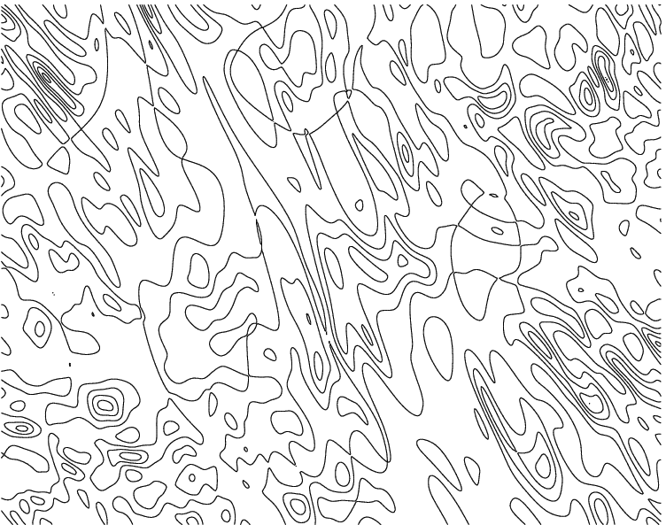
We have plotted a sample 2D section of the optimization space in Fig. 1. The axes represent two orthogonal directions in the optimization space of a certain two-qubit gate. The $x$-axis was obtained by interpolating between two known minima, whereas the $y$-axis was chosen randomly. One can readily verify from the figure that the optimization task is indeed extremely hard.

The calculation of the holonomy requires evaluating the ordered product in Eq. (8). The method used in the numerical algorithm is to simply write the ordered product in a finite-difference approximation by considering the connection components as being constant over a small difference in the parameters $\delta\gamma_{i}$, i.e.

Throughout the study we used 200 discretization points per edge, i.e., $n=200\times(k+1)$.

First we attempted to find a loop that yields the Hadamard gate.Using a random initial configuration, we obtained the results that are plotted in Fig. 2. The error function $f(\gamma)$ had a value smaller than $10^{-8}$ at the numerical optimum.The plot represents all the possible projections on two perpendicular axes (the horizontal axis is always $\theta_{1}$) in the four-dimensional space. Note that this optimization was carried out in $\mathcal{V}_{3}$, meaning that there are three vertices other than the reference point. The results do not take advantage of the $2\pi$ periodicity. We have also included the data points in Table 1. It is impressive that such a simple control loop yields the gate. Furthermore, this is just one implementation of the Hadamard gate. It is possible to find many different ones.

Another example of one-qubit gates is given in Fig. 3 and in Table 2. The gate that we tried to implement was now chosen arbitrarily to be $U=e^{i}\exp\left(i\frac{\pi}{7}\sigma_{z}\right)\exp\left(i\frac{1}{3}\sigma_{y}\right)\exp{i\sigma_{z}}$. Again, the error was well below $10^{-8}$ at the optimum. We argue that our method is capable of finding any one-qubit gate. These results are not very enlightening as such, but should nevertheless clearly prove the strength of the technique.

We also found several implementations for two-qubit gates. Figure 4 presents the loop $\gamma_{\mathrm{CNOT}}\in\mathcal{V}_{3}$ that produces the CNOT. We observe, however, that again the minimization resulted in an accurate solution. The minimization landscape is just as rough in the case of two qubits. Now, of course, the dimension of $\mathcal{V}_{3}$ is 24.

We also found an implementation of the SWAP gate given in Fig. 5.

Finally, it is interesting to observe that even the two-qubit quantum Fourier transform can be performed easily. The resulting loop is presented in Fig. 6. It is remarkable that such a simple single loop yields a two-qubit quantum Fourier transform. We used only three vertices but were still able to find an acceptable solution. We argue that the error can be made arbitrarily small for any two-qubit gate.

The realization of arbitrary one- and two-qubit gates in the context of holonomic quantum computation has been demonstrated. By restricting the loops in the control manifold within a polygon with $k$ vertices, it becomes possible to cast the realization problem to a finite-dimensional variational problem. We have shown explicitly that some useful two-qubit gates are realized by a single loop.

A possible improvement of the present scenario would be to minimize the length of the path realizing a given gate. This can be carried out by introducing an appropriate penalty or barrier function and the Fubini-Study metric in the control manifold $\mathbb{C}P^{2}$. This optimization program is under progress and will be reported elsewhere.