Energy Requirements for Quantum Data Compression and 1-1 Coding

Data compression is already a fundamental and well developed branch of classical information theory. It has wide reaching implications on every aspect of information storage and transmission and its quantum analogue is of considerable interest in a wide range of applications [2]. In quantum information theory the idea of quantum data compression, in its strictest sense, has still much to gain from the classical theory with only some of the more fundamental classical notions being translated [1, 6, 7, 8, 9].

The basis for compression of classical data is Shannon’s noiseless coding theorem [10], which states that the limit to classical data compression is given by the Shannon entropy. Schumacher [7] presented the quantum analog to this and proved that the minimum resources necessary to faithfully describe a quantum message in the asymptotic limit is the von Neumann entropy of the message $\rho$, given by $S(\rho)=-tr\rho\log\rho$. Schumacher also demonstrated that by encoding only the typical subspaces this bound could be achieved using a fixed length block coding scheme, and how in the asymptotic limit the compressed message can be recovered with average fidelity arbitrarily close to unity.

The fact that Schumacher’s scheme is only faithful in the asymptotic limit has led many to ask whether there is a scheme where we can losslessly compress in the finite case i.e. where we want to be able to compress without loss of information in the case where we have a finite (i.e. more practical) number of qubits. Of course there are many reasons why such a scenario would be desirable, e.g. in a quantum key distribution (QKD) scheme where often very high fidelity of the finite received signal is crucial to the integrity of the scheme [11]. It is in such cases that the asymptotically faithful Schumacher compression would not be ideal. This has, directly or indirectly, inspired a number of other quantum schemes [1, 8, 9] based on classical ideas of lossless coding, such as Huffman, arithmetic and Shannon Fano coding [12].

The primary consideration in lossless compression schemes is the efficient generation and manipulation of variable length codes (i.e. codes of variable rather than fixed block length). This is because (as proven in particular by Boström and Felbinger [1]) it is not possible to achieve truly lossless compression using block codes. The application of variable length codes to quantum data compression is however not quite so straightforward. The main issue seems to be that we are forbidden by quantum mechanics to measure the length of each signal without disturbing and irreversibly changing the state and resulting message. In our scheme however we show both compression and decompression to be unitary operations and there never be any need for a length measurement of the variable length states.

The main point of this paper is two fold, by looking at quantum data compression in the second quantisation, we present an entirely new model of how we can generate and efficiently use variable length codes. The significance of this model is that we believe it is a more natural application of variable length coding in quantum information theory. More importantly still is that fact that any data compression (lossless or lossy) can be seen as the minimum energy required to faithfully represent or transmit classical information contained within a quantum state. This allows us to use energy and entropy arguments to give a deeper insight into the physical nature of quantum data compression and to suggest bounds on the efficiency of our lossless compression protocol in a novel and interesting way.

The rest of this paper is broken down as follows; Section II of our paper is dedicated to reviewing the second quantisation and introducing our notation for the description of quantum states. In this description the average length of the codeword is related to the number of “modes” that are occupied. Using this fact, we look at the average energy of the message instead of its average length and therefore represent the compression limit from an energy rather than length perspective. In Section III this offers the possibility to interpret data compression in terms of the Landauer erasure principle. In Section IV we introduce a compression algorithm that uses the second quantisation to generate variable length codes and show how the need for prefix or uniquely decipherable codes is unnecessarily restrictive given the structure of quantum mechanics. The absence of this restraint leads us to the concept of one-to-one (’1-1’) codes. Classical results are then used to present an analogous quantum 1-1 entropy bound which, when taking into account the classical side information, asymptotically tends towards the existing Von Neumann bound. Finally, in Section V, we give an experimental setup for a small example that could be used to demonstrate the legitimacy of this new compression algorithm.

In this section we introduce our second quantisation notation and then show, initially using Schumacher’s scheme as an example, how data compression can be seen as the minimum energy required to faithfully represent or transmit classical information contained within a quantum state.

The general scenario for data compression is that a memoryless source, say Alice, wants to send a message $M$ to a receiver Bob, in the most ’efficient’ way possible. The efficiency of this communication in space or time may be described through the optimisation of any one of a number of parameters e.g. minimising the number of bits or the total energy required to represent the message (the two are not necessarily equal). The scenario we use in this paper is similar to that employed by Schumacher [5]. In our protocol the source Alice, wishes to communicate a number, $n$, of quantum systems (which we call the letters) prepared from a set of $N$ distinct (but not necessarily mutually orthogonal) states $|\psi_{1}\rangle,|\psi_{2}\rangle\ldots|\psi_{N}\rangle$ to Bob in the most efficient manner. It is also worth clarifying that like in Schumacher’s scheme, we consider the compression of a single source message, this is in contrast to other many message schemes with an extended memory/source set [1]. In addition in our scheme our objective is to minimise the energy of any given sequence of states generated by the source having only the probabilities of the source and indeed knowledge of the letter states themselves. Here each letter corresponds to a distinct part of the message, with $n$ letters representing the whole message. Alice then compresses this message and sends the statistical properties to Bob. Bob then adds the redundancy back into the message (using the classical side channel, as we see later) and then performs a set of transformations to determine the correct sequence of states comprising Alice’s letters, which he can then begin to use to reconstruct the entire message. This last part is known as decompression of the message. In this paper, we assume that the communication is noiseless, i.e. the states suffer no error on the way to the Bob, the letters are statistically independent from one another (i.i.d.), and for comparison with other classical and quantum compression schemes and without loss of generality that Alice communicates qubits.

There are a number of physical systems that may be used to realise qubits e.g. two different polarisations of a photon, two different possibilities for the alignment of nuclear spins in a uniform magnetic field (“up and down”), or the two energy levels of an electron orbiting say a hydrogen atom. In this paper, although our terminology for encoding and manipulating information refers to polarisations of a photon, the underlying theory and results can be conveniently applied to other qubit realisations (matter or field alike).

In addition to polarisation ($P$) let us use another degree of freedom, say frequency ($\omega$). A third possible degree of freedom is spatial location or coordinate, which will be used in section VI. Now in the second quantisation picture with the set of frequencies $\omega_{i}$, and the polarisations, $H$ or $V$ (i.e. whether the photon horizontally or vertically polarised) we can represent a system consisting of a variable number of photons by the following basis states:

Here we have $N$ different modes of the system i.e. $N$ different frequencies, $w$. Each mode is made up of 2 different harmonic oscillators, one for each polarization. It is worth noting that in our protocol these frequencies do not act as additional information carrying degrees of freedom, they are merely placeholders to distinguish the qubits and are assumed to fixed apriori by the source or sender and receiver (a good example of this is if we consider the normal modes in a cavity). That these prior correlations exist between the sender and receiver is a common and necessary part of any spatial or temporal information transfer.

Anyhow writing the system in this basis tells us that we have: $n_{1}$ photons with frequency $w_{1}$ in a horizontal polarisation, $m_{1}$ photons with frequency $w_{1}$ in a vertical polarisation and so on until $n_{N}$ photons with frequency $w_{N}$ in a horizontal polarisation and $m_{N}$ photons with frequency $w_{N}$ in a vertical polarisation. Note that states with different number of photons are orthogonal. The most general state of this system is a superposition of all the basis states above:

In practice there are infinitely many modes, but we only consider the ones which are occupied. The unoccupied modes will be said to be in a vacuum state. If our state consisted of say only $1$ vertically polarised photon in only the first mode, this could be represented as:

All of the states can be generated from the overall vacuum state or zero state (which is the one containing vacuum in every mode). They can be generated (or destroyed) by applying creation (and annihilation) operators, $a$ (and $a^{\dagger}$) respectively, where there are separate operators for both horizontally and vertically polarised photons. In general we stick to only one excitation per mode. In addition given that these modes are fixed apriori by the source or sender and receiver, there is exactly one photon in all the modes between the lowest frequency mode and the first vacuum mode. We keep to one excitation per mode to ensure that this scheme applies equally well to both bosonic and fermionic systems and keeping the scheme as universal as possible.

In this framework it is easier to see that compressing from $n$ qubits to $m$ qubits leads to a reduction in average energy. This is because in order to create or annihilate one photon in the mode $w_{i}$, requires investing or releasing an amount of energy equal to $\hbar\omega_{i}$. To see this, let us first write the Hamiltonian for this system:

which is the standard harmonic oscillator Hamiltonian for every mode and polarization, summed up over all of them independently. In this Hamiltonian the modes are independent and non-interacting. The interaction between the modes will be added later and used for data compression and decompression.

Suppose now that a quantum source randomly prepares different qubit states $|\psi_{i}\rangle$ with corresponding probabilities $p_{i}$ (keeping this analysis general we can apply this to systems of higher dimension than qubits). A random sequence of $n$ such states is produced. The question is, by how much can this be compressed, i.e. how many qubits do we really need to encode the original sequence (in the limit of large $n$)? First of all the total density matrix is

After the compression the total message would consist of some smaller number $m$ of qubits, in the state $\rho_{m}$ and it is the ratio ${m}/{n}$ that our compression aims to minimise. In the case of Schumacher’s compression this is achieved by projecting $\rho_{n}$ onto the typical subspace and then if the projection is successful the resulting strings are then encoded using a block coding scheme analogous to that employed by Shannon [10]. In the asymptotic case the probability that we are not successful in this projection goes exponentially close to zero as $n$ increases. Therefore the efficiency of quantum encoding is the same as the efficiency of the classical block coding scheme used, after the successful projection onto the typical subspace. The best way of deriving this is to look at the density matrix in the diagonal form

Now, this matrix can be diagonalised

where $r_{i}$ and $|r_{i}\rangle$ are the eigenvectors and eigenvalues. This decomposition is, of course, indistinguishable from the original one (or any other decomposition for that matter). Thus we can think about compression in this new basis, which is easier as it behaves completely classically (i.e. they are fully distinguishable since $\langle r_{i}|r_{i}\rangle=\delta_{ij}$). We can therefore invoke results from Shannon’s work on classical typical sequences [10] to conclude that the limit to compression is $n(-\sum_{i}r_{i}\ln r_{i})$, i.e. $n$ qubits can be encoded into $nS(\rho)$ qubits. No matter how the states are generated, as long as the total state is described by the same density matrix $\rho$ its compression limit is its von Neumann entropy.

We now want to show briefly that this is the same as the ratio of the initial and final energy in the second quantisation and data compression is therefore the same as energy reduction in our communication framework. The average initial (before compression) and final (after compression) energies in our message are defined by the usual trace rule:

Asymptotically we claim that:

We now substantiate this claim and a slight change in notation will make this easier to see. We define a message of length $n$ to be described by the density matrix $\rho_{n}=\rho_{i}^{\otimes{n}}=(\sum_{i=1}^{n}p\left(\psi_{i}\right)\left|\psi_{i}\right\rangle\left\langle\psi_{i}\right|)^{\otimes n}$, which again when written in the diagonal basis gives:

this is equal to

For large $n$, the number of times the ket $|r_{j}\rangle$ appears is, as a consequence of the law of large numbers, $nr_{j}$.

Without loss of generality this proof looks at a source, Alice, generating photons in only one of two states at a time, $|\psi_{1}\rangle$ or $|\psi_{2}\rangle$ where the state $|\psi_{1}\rangle=a|H\rangle+b|V\rangle$ and $|\psi_{2}\rangle=a|H\rangle-b|V\rangle$. Each generated photon corresponds to a letter of the message, where the whole length of the message is measured in qubits. The overlap between the two states is $a^{2}-b^{2}$ and if $b=\sin(\theta/2)$ and $a=\cos(\theta/2)$ this overlap becomes $\cos\theta$. Therefore our two eigenstates are:

which when looked at in the second quantisation framework can be rewritten as:

A compression-decompression scheme of rate $R$ consists of two quantum operations ${C}^{\prime}$ and ${D}^{\prime}$ analogous to the maps defined for the classical case [12] where the compression operation ${C}^{\prime}$ is taking states from $H^{\otimes n}$ to $H^{\otimes nR}$ and the decompression ${D}^{\prime}$ returns them back. One can define a sequence $r_{i_{1}}r_{i_{2}}r_{i_{3}}\cdots r_{i_{n}}$ as $\epsilon$-typical by a relation similar to the classical

This is a rigorous statement of the law of large numbers [12]. A state $\left|r_{i_{1}}\right\rangle\left|r_{i_{2}}\right\rangle\cdots\left|r_{i_{n}}\right\rangle$ is said to be $\epsilon$-typical if the sequence $r_{i_{1}}r_{i_{2}}r_{i_{3}}\cdots r_{i_{n}}$ is $\epsilon$-typical. The $\epsilon$-typical subspace will be noted $T\left(n,\epsilon\right)$ and the projector onto this subspace will be:

By using a block coding scheme to encode only the typical subspace, Schumacher manages to compress the message from $n$ to $m$ qubits, so that the state is:

Writing this in our representation, this means that only the first $m$ modes are populated, the other $n-m$ modes being empty. Schumacher proved that in the asymptotic limit the average number of qubits required tends to the Shannon entropy. Therefore from our energy perspective we can say that, as originally each qubit corresponds directly with a mode containing a photon, on average we are saving $n-m$ photons. Assuming all photons have the same energy of $\hbar\omega$ (i.e. all the modes have the same frequency and energy is the same for both $H$ and $V$ polarisations) then the following is true:

With regards to the assumption that all photons are of the same energy, for this proof we can for example practically assume that the frequencies are very close to each other (emitted from a large cavity). Not only that, but we can also assume that we always emit a photon from the same mode - but then the spatial component (equivalently the temporal component) of all these would be different which is how we could discriminate them. Anyhow following on from this, therefore:

From Schumacher, the ratio $m/n$ we know to be equal to $S(\rho_{n})$. The entropy therefore tells us not only how much information can be compressed but also how much energy is used for computation. In the Schumacher block coding scheme [5] the average message length divided by the final message length gives us the entropy. Given that for us the average message length is the number of kets that are non zero, it makes more sense to look at average energy rather than average length. In this way we reinterpret the entropy from an energy rather than length perspective.

Note that here we used Schumacher’s compression to illustrate how compression works, but any other compression scheme would also amount to energy reduction. In fact in section IV we will present a scheme completely different to Schumacher’s (i.e. faithful for any finite length of message) which can also be regarded as reducing the energy of the original message whilst preserving its information content. A conceptual advantage of our formulation is that we have a more physical interpretation of data compression through Landauer’s erasure, which we look at next.

We can also show how Landauer’s principle [16] can be used to derive the limit to quantum data compression. This principle states that in order to delete a message containing entropy S, it is necessary to use kT S energy. In particular this means that in order to delete 1 bit of information from some message you need to generate at least one bit of entropy (heat) in the environment of the message. In order to see this suppose that the qubit to be deleted is in the maximally mixed state $I_{m}/2$. We know there is no unitary (reversible) transformation that maps this into a pure state. The best that we can do is swap a clean pure qubit from the environment with the maximally mixed one to be deleted [15].

where the swap transformation is defined as:

In this way the entropy of $1$ (qu)bit that existed in the system is now transferred to the environment as since the whole transformation is at best unitary (reversible) we can see that the environment cannot increase in entropy by less than $1$ (qu)bit. This is the key observation of Landauer’s principle. If the qubit that we are erasing is originally entangled to another qubit of the message, then after the swap operation with the environment, the corresponding environmental qubit becomes entangled with the message (This is the simplest instance of the so called entanglement swapping scheme and will be exploited in our later implementation of our own data compression algorithm scheme). Note that there are several ways of formulating this principle. It could be phrased in terms of entropy or in terms of free energy or even in terms of the heat that is generated. These are all equivalent. All this thermodynamical reasoning applies in the so-called thermodynamical limit, i.e when we manipulate a large number of systems (in our case this means a sufficiently long message).

The fact that we release energy but do not lose any information is fundamental to lossless quantum data compression. By controlling the release of ’redundant energy’, that carries no information we can keep the quantum coherences intact. If no information is lost during compression the two free energies (or entropies) before and after the compression should be equal (c.f. [14]). If we generated less heat after compression, this means that there was less information to delete - implying that our compression was not faithful (and vice-versa). Therefore if $n$ qubits in a state $\rho$ are compressed to $m$ qubits in a state $\sigma$ the most efficient compression according to Landauer’s erasure would result in $nS(\rho)=mS(\sigma)$. In order to minimise $m/n$ (i.e. achieve the most efficient compression) the entropy of the encoded bits should be maximal, $S(\sigma)=1$ implying that $\sigma$ has to be in a maximally mixed state. Since we know Landauer principle has to be obeyed, if the compressed message generates a lower amount of heat when deleted this implies that in order to decompress this message we need another piece of information about it to make up the difference between Landauer’s heat and this heat. We will see an example of this in the next section when we introduce our own coding scheme.

We have seen that Schumacher’s encoding is lossy for a finite length of message and that it only becomes faithful in the asymptotic limit. Now we present an encoding which is faithful for any number qubits. Our encoding compresses the quantum information in the qubits beyond the von Neumann limit, but at the expense of having to send an additional piece of (classical) information about the state from source. We will see how when adding both pieces of information together the efficiency of our compression scheme, like Schumacher’s, tends asymptotically to the Von Neumann limit. To see how this can be achieved, suppose again that a quantum source randomly prepares different qubit states $|\psi_{i}\rangle$ with the corresponding probabilities $p_{i}$ (keeping this analysis general we can apply this to systems of higher dimension than qubits). A random sequence of $n$ such states is produced. The question is then how many qubits do we really need to encode the original sequence i.e. by how much can the source be compressed?

As before the single-shot density matrix for the source is:

If we assume we know the probability distribution $p_{i}$ (for all $i$) of the source then this matrix can be diagonalised to give

where $r_{i}$ and $|r_{i}\rangle$ are the eigenvectors and eigenvalues. The advantage of diagonalisation is that compression in this new basis is easier as the state behaves completely classically (since $\langle r_{i}|r_{i}\rangle=\delta_{ij}$). We can then invoke results on classical compression methods to compress the resulting state. The important difference here to other compression schemes with an extended memory/source set [1] is that by considering compression in the second quantisation we have a novel framework for implementation of variable length codes. We will first introduce our scheme through an example and then discuss its generalization and efficiency.

The interesting thing here is that classically it is not possible to compress a source that generates $0$ and $1$ with equal probability. Quantum mechanically, however, compression can be achieved not only by the nature of the probability distribution but also due to the non-orthogonality of the states encoding symbols of the message. In this example the overlap between the two states is $\langle\psi_{0}|\psi_{1}\rangle=\sin\theta$ and they are orthogonal when $\theta=\pi$. Essentially the smaller the overlap, the more the total message can be compressed. This can also be expressed in terms of information, as the smaller the overlap, the less distinguishable the states and hence the less information they carry.

As Alice’s message is only $3$ qubits long. Then there are $8$ different possibilities, $|\Psi_{0}\Psi_{0}\Psi_{0}\rangle,...|\Psi_{1}\Psi_{1}\Psi_{1}\rangle$, which are all equally likely with $1/8$ probability.

It is always possible to go to a basis where the density matrix is diagonal (here we are using the first quantisation notation for clarity):

where $|\pm\rangle=|0\rangle\pm|1\rangle$. Consequently for 3 qubits:

By rewriting the combined state in the second quantisation and making use of the fact that the only requirements on the resulting codeword is that it is unique (i.e. 1-1) we can encode our message as follows:

where $a=[\frac{(1+sin\theta)}{2}]$, and $b=[\frac{(1-sin\theta)}{2}]$. Of course the states appear to be of different length but as we explained in Section II this is not the case, the missing modes are occupied by vacuum states (which carry no information). The logic of our compression is that the state with the highest probability (the one that appears most in the classical language) is encoded in the shortest possible form. Note that this is different to Schumacher’s strategy. Schumacher only encodes the states in the typical subspace, and all the other states are deleted (leading to unfaithful compression for the finite size message). The states in the typical subspace, on the other hand, are in Schumacher’s case all encoded into codewords of equal length (asymptotically equal to the original length times the entropy of the signal). In our scheme the typical subspace does not have exclusive importance, with all the messages being encoded faithfully. Note finally that the whole transformation is unitary and therefore can be implemented in quantum mechanics (we show how to do so in section V).

From this encoding, when say, $\theta=45^{\circ}$, we can infer the entropy of the string as $1.29$ bits/symbol. This is better than our expected optimal of $1.8$ bits/symbol and is a significant improvement on Schumacher codings $1.88$ bits/symbol. However, as we will see, it is not appropriate and is actually misleading to directly compare these results without the added the respective information required from the classical side channel. The main advantage of this compression method over that of Schumacher’s is that this is lossless in the finite case, i.e. signal can be completely recovered, unlike in Schumacher’s case where a certain loss in fidelity is inevitable. It is clear that our example with $3$ qubits can in fact be applied to any number of qubits (or, more accurately, to quantum systems of any dimension) by continuing with the principle of encoding less likely strings into states with more photons. This mapping is perfectly well defined and unique even given the case that we have messages of equal probability, where here we can arbitrarily choose which message to encode into the shorter word.

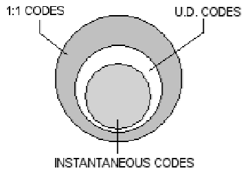
An important point to make is that in this scheme we no longer need to use the classical notion of unique decipherability (Fig 3)[12, 13] for defining codeword mappings. This is because given the encoding technique any codeword set that represents a 1-1 map between codeword and letter state is sufficiently effective in being uniquely decipherable (U.D.). Therefore the quantum notion of U.D., as directly applied in this case, is stronger and allows for shorter codewords than is classically possible, something that has has also been considered by Boström [1].

In terms of decompression, classically we make use of the fact that we have the length information of each codeword. However in quantum mechanics encoding the length information of each codeword along with the respective codeword is quite impractical, as a number of authors have pointed out [1, 3, 6]. This is because in quantum mechanics in order to infer the individual length of a codeword would require there to be a measurement of some sort and performing any measurement would collapse this superposition onto any one of those codewords irreversibly, resulting in a disturbance to the state and therefore an unacceptable loss of information. It is therefore indeed fortunate that in order to faithfully decompress (i.e. replace the redundancy that was removed by quantum compression) we need only to know the total length of the message that was initially encoded (i.e. total number of qubits transmitted) rather than the individual lengths of each codeword (i.e. length of each letter state). With having only this total length information, $l_{t}$ we then know the redundancy we need to add to the compressed signal (i.e. the signal containing the statistical properties of the original message) in order to restore the original message. Clearly if this information is missing we can only probabilistically achieve faithful decompression by best guessing the original length of the message as also pointed out by Boström [1]. As $l_{t}$ cannot be measured, it must be known by the sender and sent additional to the compressed quantum message (see Fig. 4)(via a classical or quantum side channel) or perhaps agreed upon between sender and receiver prior to communication. It is worth clarifying that classically, $l_{t}$ is always available to us regardless of the coding scheme employed, as we can easily make a measurement on its length without any risk of disturbing the state.

From Landauer’s erasure principle [16], briefly discussed and applied in section III, it is possible to derive an lower bound on the efficiency of this compression scheme. We use the fact that according to Landauer when we erase n units of information we have to increase the entropy of the environment by n units. If the entropy increase of the environment is less than this, that then must imply that there is a suitable amount of information that was not deleted.

The encoding we use to achieve compression is faithful for any finite length of message, only if, as mentioned before, together with the compressed message we send another piece of information. This could be the total length of the uncompressed message, or instead, slightly more efficiently, the entropy of the message. So, if the statistical properties of the message are represented by $\rho_{n}$, we could send additional $\log n$ (qu)bits along with the compressed message to represent the length of the total signal, or, at best send $\log S(\rho_{n})$ (which is $\leq\log n$). Therefore from Landauer’s principle we expect that the limit to compression in our scheme is bounded from below by:

if we are sending log(n) bits of length information or

if we, more efficiently, only send the entropy of the total signal, from which it is possible to infer the length information.

In this section we discuss practical issues related to realising a a very simple instance of our 1-1 quantum encoding scheme. We will be encoding two quantum bits in the state $|\psi_{0}\rangle$ or $|\psi_{1}\rangle$ where as in the earlier 3 qubit example $|\Psi_{0}\rangle=\cos(\theta/2)|0\rangle+\sin(\theta/2)|1\rangle$ and $|\Psi_{1}\rangle=\sin(\theta/2)|0\rangle+\cos(\theta/2)|1\rangle$ with $p_{0}=p_{1}=1/2$. As in the 3 qubit example, going into the basis where the density matrix is diagonal and then mapping the respective letter states to corresponding codewords in order of most probable to least probable (again here assuming $a>b$), we get:

Note that this operation just tells us to annihilate the second photon if it is the state $|+\rangle$ and map $|+\rangle$ to $|1_{H},0_{V}\rangle$ and $|-\rangle$ to $|0_{H},1_{V}\rangle$. So in order to implement this transformation we clearly need to be able to perform a conditional operation from the polarisation degrees of freedom to the spatial degrees of freedom. The subsequent transformation is then just a change of basis, from a $+/-$ basis to a $H/V$ basis, which is known as the Hadamard transform and is easy to implement. We know that as we have an orthogonal set on the left hand side and an orthogonal set on the right hand side, according to quantum mechanics there must be a unitary transformation to implement this. Since Hadamard is a simple transformation to implement we only need to show how to implement the following two qubit transformation:

which actually amounts to deleting the second photon if its state is $H$ and otherwise leaving everything the same. Note that, due to linearity of quantum mechanics, a superposition of states on the left hand side would be transformed into the corresponding superposition of the states on the right hand side. This means that we will have elements of unequal length (different number of photons) present in the superposition. While this may in practice be difficult to prepare, there is nothing fundamental to suggest that in principle such states cannot be prepared, as we show next.

In order to implement this transformation, one possible method is presented in Fig. 5 in the form of a simple quantum computational network. In this circuit, we first need to distinguish the two modes as we only want to delete a particle from the second (and not the first) mode. We can imagine that in practice if these are two light modes, then we actually need to distinguish their frequencies $\omega_{1}$ and $\omega_{2}$, and this could be done by a prism splitting the two frequencies at A. Therefore the two modes now occupy different spatial degrees of freedom. Next we need to distinguish the two polarisations in the second mode, which in the case of a photon would involve a polarisation dependent beam splitter (PDBS) at B. Now, after this beam-splitter we can distinguish both the frequency and the polarization in the second mode, and so we only need to remove a photon from the second mode if we have H polarization. Here we use the trick we mentioned in the Landauer’s erasure section, namely that we swap the photon in the second mode with an environmental vacuum state conditional on it being horizontally polarized (and otherwise we do nothing). If initially we had a superposition of all states $a|1_{H},0_{V}\rangle|1_{H},0_{V}\rangle+b|0_{H},1_{V}\rangle|1_{H},0_{V}\rangle+c|1_{H},0_{V}\rangle|0_{H},1_{V}\rangle+d|0_{H},1_{V}\rangle|0_{H},1_{V}\rangle$, and the state of the environment was $|0_{H},0_{V}\rangle$, then after the swap, the state will be

We now need to perform a simple Hadamard transformation on the environment such that

after which the total state can be written as

Note that after performing a measurement on the environment (at C), if we obtain the outcome $|0_{H},0_{V}\rangle$, then the resulting state of two photons is already our encoded state, while if the outcome is $|1_{H},0_{V}\rangle$, then the state is the encoded state up to a negative phase shift in the last two elements of the superposition. This can be corrected by applying a simple phase shift conditional on the second photon being vertical. The whole operation at C can also be performed coherently without performing the measurement as indicated in Fig 5. We acknowledge that this operation may not be simple to execute in practice and may require a $100$ percent effective photo-detection scheme which is currently unavailable. However, this gate can certainly be implemented with some probability at present. At the end, we need to reverse the operation of the PDBS, and then reverse the operation of the prism, thus finally recombining the two modes into the same spatial degree of freedom. The resulting state is our encoded state and can then be sent as such.

In this paper a new variable length quantum data compression scheme has been outlined. By looking at quantum data compression in the second quantisation framework, we can generate variable length codes in a natural and efficient manner without having the significant memory overhead common to other variable length schemes [1]. The quantum part of our signal is compressed beyond the von Neumann limit, but at the expense of having to communicate a certain amount of classical information. By sending the total length of the transmitted signal through a classical channel enables us to compress and decompress with perfect fidelity for any number of qubits. We have presented an argument based on Landauer’s erasure principle which provides us with a with a lower bound on the efficiency of our compression scheme. This is independently verified by classical results due to Cover [17] and Prisco [18]. As expected, the sum of the classical and the quantum parts of the compressed message still tends towards the limit given by the von Neumman entropy. Asymptotically, the quantum part dominates over the classical part and becomes equal to the von Neumman entropy. The tightest compression bound for our scheme is not known.

Note that we assume that both the sender and receiver know exactly the properties of the source, i.e. they know the quantum states the source emits and the corresponding probabilities and modes within which they are emitted. This of course means that our scheme is not universal. It is unlikely however that in a universal scheme the sender and receiver would need less information than this to perform compression, e.g. just knowledge of the entropy of the source and length of message without knowledge of the density matrix (or perhaps even this is unnecessary [19]). But this is a separate issue that warrants further investigation.

Our encoding has a novel feature that it involves superpositions of different numbers of photons within the superposition states. We acknowledge that there may be a “superselection” rule that prohibits the nature of this approach. However, we believe that, while these states might be difficult to prepare, they are certainly not impossible according to the basic rules of quantum mechanics. To support this we offer a general way of implementing our scheme in the simple case of encoding two quantum bits. Whether the space-time complexity of our implementation is most efficient in practice remains an open question.

As it is, our encoding is a unitary transformation and the receiver applies the decoding operation (inverse of the unitary transformation) to decompress the quantum message. In the case that we encode and send classical bits, the receiver may wish to infer the original classical string that was sent. The receiver can then perform measurements on the decompressed quantum states to infer the original classical letters. Since the original classical letters are by definition fully distinguishable and if the transmitted quantum states are orthogonal only then can this final step be done with perfect efficiency (this is of course a special case of our most general quantum scheme).

It is also worth noting that it is on the sequence of these quantum states i.e. on the total message, that our compression scheme acts. This means that this scheme would not be so useful in an application where instantaneous lossless decompression is required, where one would have to wait for all the photons to arrive before beginning the decoding operation. In the event that the receiver starts the decompression operation in advance of the last photon arriving, he truncates the signal and hence will not be able to decode the original signal with perfect fidelity.

In our scheme it is the average length of the message, or more appropriately the average energy required to represent the information within the quantum state, that tends in the asymptotic limit towards the von Neumann entropy. We therefore decided instead to re-formulate compression from an energy perspective, as the measure is then more consistent as an optimal measure of a systems information carrying ability. As we are aware in quantum mechanics, energy and information are intricately linked, far more so than photon number and information. We are interested in primarily reducing the energy required to represent the message, which we stress is not affected by the fact that we need to wait until the whole signal is received. In our framework the incorporation of any vacuum states to extend the variable length message to the same length as the longest component of the superposition, by definition, does not increase the energy total for the message. In reality of course we do not even have to wait for the whole signal, we can just truncate it at the average length of the signal and although we end up with a lossy compression scheme we still tends towards the von Neumann entropy asymptotically. The issue of waiting until the whole signal arrives really is to do with the fact that we cannot measure the length of the signal without collapsing it into a particular length, which is not what we want as we want to keep intact the superposition and consequently preserve the rest of the information within the system.

Our approach raises a number of interesting questions. Firstly, it gives us a more physical model of data compression and relates the entropy to the minimum energy required to represent the information contained within a quantum state. This could be very useful from an energy saving perspective and gives a guideline as to the minimum temperature we could cool a system to before we begin to loose information. Another benefit to this compression scheme is that it does not depend on the nature of particles, the scheme applies equally well to both bosonic and fermionic systems. The reason for this is that we never put more than one particle per state when we are encoding and therefore we never need to consider the Pauli exclusion principle. Whether this principle plays a more important role in data compression, i.e. whether there could be a fundamental difference between the bosonic and fermionic systems ability to store (and in general process) information is not yet known. The ultimate bound due to Bekenstein [20] suggests that the answer is “no”, however, specific encodings may highlight differences between the two kinds of particles.

Finally, our scheme assumes that the encoding and the decoding processes as well as the possible channel in between the two are error free. In practice this is, of course, never true and it is interesting to analyze to what extent our scheme suffers in the presence of noise and decoherence at its various stages. We hope that our work will stimulate more research into quantum data compression as well as experimental realization in the optical and the solid state domain.

We would like to acknowledge useful discussions with K. Boström, D. Bouwmeester, G. Bowen, C. Rogers and useful communication with T. Cover and J. Keiffer. L. R. acknowledges financial support from Invensys plc. V.V. would like to thank Hewlett-Packard, Elsag s.p.a. and the European Union project EQUIP (contract IST-1999-11053) for financial support.

References

- [1] K. Bostroem and T. Felbinger. ”Lossless Quantum Data Compression and Variable Length Coding”. Phys. Rev. A 65, 032313 (2002).
- [2] V. Vedral, Rev. Mod. Phys. 74, 297 (2002).
- [3] R. Cleve, D. DiVicenzo. ”Schumacher’s Quantum Data Compression as a Quantum Computation”. Phys. Rev. A 54, 2636 (1996).
- [4] S. Bose, L. Rallan and V. Vedral. ”Communication Capacity of Quantum Computation”. Phys. Rev. Lett. 85, 5448 (2000).
- [5] B. Schumacher. “Quantum Coding”. Phys. Rev. A 51, 2738 (1995).
- [6] B. Schumacher and M.D. Westmoreland. “Indeterminate Length Quantum Coding”. Phys. Rev. A 64, 042304 (2001).
- [7] R. Jozsa and B. Schumacher. ”A New Proof of the Quantum Noiseless Coding Theorem”. J. Mod. Opt. 41, 2343 (1994).
- [8] I.L. Chuang and D.S. Modha. ”Reversible Arithmetic Coding for Quantum Data Compression”. IEEE Transactions on Information Theory, 46, (2000).
- [9] S. Braunstein, C.A. Fuchs, D. Gottesman, and H.-K. Lo. ”A Quantum Analog of Huffman Coding”. IEEE International Symposium on Information Theory (1998). quant-ph/9805080 (1998).
- [10] C. E. Shannon and W. Weaver, “The Mathematical Theory of Communication”, (University of Illinois Press, Urbana, IL, 1949).
- [11] M. A. Nielsen and I.L. Chuang, “Quantum Computation and Quantum Information”. Cambridge University Press (2001).
- [12] T. M. Cover and J. A. Thomas. ”Elements of Information Theory”. Wiley, New York, (1991).
- [13] G.A. Jones and J.M. Jones. ”Information Theory and Coding”. Springer, London (2000).
- [14] R.P Feynman, “Feynmann Lectures on Computation”, edited by A. J. G. Hey and R. W. Allen, Addison-Wesley Publishing Company, Inc., (1996).
- [15] V. Vedral, ”Landauer’s Erasure, Error Correction and Entanglement”. Proc. Roy. Soc. Lond. A Mat. 456, 969-984 (2000).
- [16] R. Landauer, IBM J. Res. Develop. 5, 183 (1961).
- [17] S.K. Leung-Yan-Cheong and T.M. Cover. “Some Equivalences Between Shannon Entropy and Kolmogorov Complexity”. IEEE Transactions on Information Theory, 24, 331, (1978).
- [18] C. Blundo and R.D. Prisco. ”New Bounds on The Expected Length of 1-1 Codes”. IEEE Transactions on Information Theory, 42, 246, (1996).
- [19] C. Rogers, private communication.
- [20] J. D. Bekenstein, “Entropy content and information flow in systems with limited energy”, Phys. Rev. D 30, 1669, (1984).