I-concurrence and tangle for isotropic states
Abstract
We discuss properties of entanglement measures called I-concurrence and tangle. For a bipartite pure state, I-concurrence and tangle are simply related to the purity of the marginal density operators. The I-concurrence (tangle) of a bipartite mixed state is the minimum average I-concurrence (tangle) of ensemble decompositions of pure states of the joint density operator. Terhal and Vollbrecht [Phys. Rev. Lett. 85, 2625 (2000)] have given an explicit formula for the entanglement of formation of isotropic states in arbitrary dimensions. We use their formalism to derive comparable expressions for the I-concurrence and tangle of isotropic states.
I Introduction
Entanglement among quantum systems is a distinctive feature of quantum mechanics Einstein1935; Bell1964; Wootters2001 and an indispensable ingredient in various kinds of quantum information processing protocols Lo1998; Mnielsen2000, e.g., quantum teleportation. It is desirable to have a general theory of entanglement, but though important results have been obtained, a general theory has proven elusive because of the complex nature of entanglement for all but the very simplest joint quantum systems. Several measures of entanglement have been suggested and investigated: the entanglement of formation Bennett1996; Cbennett1996, the entanglement of distillation Bennett1996; Cbennett1996, the relative entropy Vedral1996; Vedral2002, the robustness of entanglement Vidal1999, and others. In this paper we explore a measure of entanglement called the I-concurrence, which was introduced by Hill and Wootters Hill1997; Wootters1998 for pairs of qubits and generalized to arbitrary bipartite systems by Rungta et al. Rungta2001. Before turning to the I-concurrence, we summarize here relevant results from entanglement theory which will facilitate the discussion of I-concurrence.
Work on entanglement has served to identify certain a priori axioms for a good measure of entanglement Vidal2000. Entanglement characterizes intrinsically quantum-mechanical correlations between quantum systems. If denotes an amount of entanglement in the joint state of several quantum systems, a fundamental requirement for to be a good measure of entanglement is the following:
- 1.
does not increase, on average, under local operations and classical communication (LOCC). Such a measure is called an entanglement monotone Vidal2000.
An entanglement monotone must remain the same under the action of reversible LOCC. Hence, it is invariant under local unitary transformations since these can be locally reversed. Moreover, any state can be converted into any separable state using LOCC; therefore, an entanglement monotone takes a common minimum value for all separable states, which can always be adjusted to zero Vidal2000. Thus we can impose an additional, nonnegativity requirement for a good entanglement measure:
- 2.
and goes to zero if and only if is a separable state.
Henceforth, we restrict our discussion to bipartite quantum systems. In three or more Hilbert-space dimensions, more than one measure is required to characterize the entanglement of bipartite states Vidal1999; Vidal2000; Vidal1999b: to specify completely a joint pure state of a system, up to local actions, requires independent Schmidt coefficients. Vidal Vidal2000 showed how to construct an infinite family of entanglement monotones for bipartite systems. This family of entanglement measures, denoted by , is characterized by the following conditions.
- (i)
For a pure state , the measure is a function of the marginal density operator , i.e., , where the function has the following properties: (a) invariance under unitary transformations, i.e., , which implies that is a function of the eigenvalues of , and (b) concavity, i.e., , where , and .
- (ii)
For a mixed state , the measure is defined to be the convex-roof extension of the pure-state measure, i.e., the minimum average value of the measure over all ensemble decompositions of :
(1)
Vidal Vidal2000 showed that if a measure belongs to the above family, it satisfies property and thus is an entanglement monotone. The I-concurrence, as we show in Sec. II, belongs to this family. Vidal also showed that when restricted to pure states, any entanglement monotone satisfies condition (i).
A privileged example of an entanglement monotone comes from choosing the unitarily invariant concave function of condition (i) to be the von Neumann entropy, . This entanglement measure plays a special role because of the asymptotic reversibility of the processes of entanglement dilution and concentration for pure states, with von Neumann entropy entering as the currency for these reversible transformations Popescu1997: Bell states can be converted by LOCC to copies of in the limit as goes to infinity and vice versa Bennett1996. The corresponding entanglement monotone for pure states, , when extended to mixed states by the convex roof, is called the entanglement of formation Bennett1996; Cbennett1996:
| (2) |
Unlike the situation for pure states, however, it is not known whether the entanglement of formation gives the asymptotic cost in Bell states for creating many copies of a mixed state using LOCC. This identification depends on whether is additive Wootters2001; Wootters1998. Though is additive on pure states, this only implies that is subadditive on mixed states. If is strictly subadditive, then some other entanglement monotone, given by the von Neumann entropy for pure states, but less than for mixed states, quantifies the asymptotic cost of creating many copies of a mixed state Wootters2001; Hayden2001.
The special role of von Neumann entropy has been reconciled with the existence of many other entanglement monotones by Vidal Vidal2000 and Nielsen Nielsen2000. Vidal considered a class of entanglement monotones that are additive on pure states and showed that they have different asymptotic properties than the entanglement of formation. Nielsen formulated a precise property of asymptotic continuity that is satisfied by the von Neumann entropy and showed that this property is the key to relating entanglement monotones to the asymptotic reversibility of entanglement dilution and concentration that holds for pure states. Indeed, Nielsen showed that any entanglement monotone that is additive on pure states and that satisfies his asymptotic continuity property is given, for pure states, by the von Neumann entropy of the marginal density operator. This result of Nielsen’s leaves open the question of the entanglement cost for mixed states.
Entanglement monotones other than the entanglement of formation, though they are not related to asymptotic transformations, are nonetheless important for characterizing LOCC transformations between finite numbers of copies of states. Indeed, they have been used to quantify the probability and fidelity of exact and approximate LOCC transformations between pure states Vidal1999b; Nielsen1999; Jonathan1999a; Vidal2000b. In this paper we investigate the properties of entanglement monotones related to a particular entanglement measure called the I-concurrence.
Hill and Wootters Hill1997 introduced the concurrence as a measure of entanglement for pairs of qubits. The concurrence for a pure state of two qubits is defined with the help of the qubit spin-flip operator, and it is extended to mixed states as the convex roof. Wootters Wootters2001; Wootters1998 went on to derive an explicit formula for concurrence of an arbitrary joint state of two qubits in terms of the eigenvalues of , where is obtained by spin flipping , and showed how to calculate the corresponding entanglement of formation from the concurrence.
Rungta et al. Rungta2001 generalized the notion of concurrence to pairs of quantum systems of arbitrary dimension. This generalized concurrence for a joint pure state of a system is simply related to the purity of the marginal density operators:
| (3) |
The generalized concurrence is known as the I-concurrence because it is defined in terms of the universal-inverter superoperator Rungta2001, which was shown to be a natural generalization to higher dimensions of the spin flip for qubits. For the purposes of this paper, we need not introduce the universal inverter, simply taking Eq. (3) as the definition of the I-concurrence for pure states. The I-concurrence is extended to mixed states by the convex roof:
| (4) |
For pairs of qubits, Coffman, Kundu, and Wooters Coffman2000 called the tangle of the state . In this paper we prefer to refer to simply as the squared I-concurrence and to reserve the term tangle for the quantity obtained by extending to mixed states by the convex roof:
| (5) |
Osborne Osborne2002 has calculated the tangle of rank-2 density operators in systems. As noted by Osborne, the definition of tangle in Eq. (5) does no violence to the original usage of Coffman, Kundu, and Wootters, because for bipartite qubit states, the reason being that all pure states in the optimal ensemble decomposition have the same concurrence. Osborne found the tangle as defined in Eq. (5) to be a more natural quantity in his analysis of rank-2 density operators, just as we find it to be more natural for isotropic states in our analysis below.
The motivation for this paper is to show that, like the entanglement of formation, the I-concurrence and tangle are entanglement monotones (Sec. II) and then to provide explicit formulae for the I-concurrence and tangle of isotropic states (Sec. III). For our analysis of isotropic states, we use the formalism developed by Terhal and Vollbrecht Terhal2000 to calculate the entanglement of formation for isotropic states. We find that the tangle for isotropic states is closely related to the corresponding entanglement of formation (Sec. IV).
II Properties of I-concurrence and tangle
Henceforth, we will omit the “I” when referring to the I-concurrence. Consider the Schmidt decomposition of an arbitrary joint pure state of a system:
| (6) |
The squared Schmidt coefficients, , are the eigenvalues of the marginal density operators, and , of the two systems, and the vectors and make up the orthonormal bases that diagonalize the marginal density operators. These bases are connected to a fiducial orthonormal basis by unitary transformations and . The state is specified by its Schmidt vector and the unitary operators and .
The tangle, or squared concurrence, of the pure state [see Eq. (3)] is given in terms of the Schmidt coefficients by
| (7) |
is conserved under by local unitary transformations because it is a function only of the Schmidt coefficients [property (i)a]. It varies smoothly from , for pure product states, to , where , for maximally entangled pure states.
That is a concave function of () [property (i)b] follows from the fact that , , is a concave function, since for any concave function , the mapping is concave Wehrl1978). To see this, let , with and , and let , , and be eigendecompositions. Then we have
| (8) | |||||
where the two inequalities follow from the concavity of . Since adding a constant and multiplying by a positive constant doesn’t change concavity, is a concave function of . Since satisfies property (i), its extension (5) by the convex roof to give the tangle of mixed states is an entanglement monotone.
The square root being an increasing concave function, it preserves concavity. Thus the concurrence is also a concave function of , and its extension (4) to give the concurrence of mixed states is an entanglement monotone. Notice that since is zero if and only if is a pure product state, and are zero if and only if is separable.
From the properties of an entanglement monotone or directly from the convex-roof construction, it is clear that the concurrence is a convex function of bipartite density operators. Since the square is an increasing convex function, it preserves convexity, thus making the squared concurrence, , a convex function of bipartite density operators. As a convex function that agrees with the convex roof on pure states, the squared concurrence is guaranteed to satisfy . We are unable to say whether is itself an entanglement monotone, although it seems unlikely that it satisfies the property of not increasing under local measurements.
III Tangle and concurrence of isotropic states
III.1 Isotropic states
In this section we derive the tangle and concurrence of isotropic states. At the end of the section, we compare our results with the those for the entanglement of formation of isotropic states obtained by Terhal and Vollbrecht Terhal2000. The tangle of isotropic states shares important features with the entanglement of formation, but the concurrence is significantly different.
Isotropic states are a class of mixed states for systems (two qudits); they are convex mixtures of the maximally mixed state, , with a maximally entangled state,
| (9) |
Such mixtures can be expressed as
| (10) |
where , satisfying , is the fidelity of and . These states were shown to be separable for Rungta2001b; Horodecki1999.
The isotropic states are special in the sense that they are invariant under the action of the twirling superoperator Horodecki1999:
| (11) |
Indeed, the twirling superoperator reduces any two-qudit state to an isotropic state
| (12) |
where is the fidelity of and . Twirling the pure state of Eq. (6) yields an isotropic state
| (13) |
where the fidelity is given by
| (14) | |||||
being a unitary matrix. It is easy to see that
| (15) |
since ; equality holds if and only if .
III.2 Reduction to a single extremization
We turn now to finding the tangle and concurrence of isotropic states, using the technique developed for entanglement of formation by Terhal and Vollbrecht Terhal2000. We proceed with the analysis in terms of the tangle. The reader should note that nothing would change in the analysis if we replaced pure-state tangle with pure-state concurrence , thus analyzing instead of , till we get to Sec. III.4. At that point, we explicitly note the differences between the results for tangle and concurrence.
The tangle of an arbitrary bipartite state satisfies the following inequality,
| (16) | |||||
| (17) |
The inequality in Eq. (17) follows because an optimal decomposition of , i.e., one which achieves the minimum in Eq. (16), automatically generates a set that satisfies the constraint in Eq. (17). In contrast, a set that achieves the minimum in Eq. (17) generally does not generate an ensemble decomposition of . Additional simplification is achieved by splitting the minimization in Eq. (17) into two parts, i.e.,
| (18) |
with
| (19) |
The function defined in Eq. (18) is a function of the single parameter .
We can reduce the minimization problem further by noting that if is the vector of Schmidt coefficients that provides the minimum for , then [Eq. (15)] and
| (20) |
We find an explicit expression for below and show that it is monotonically increasing, from which it follows that
| (21) |
Applying Eq. (21) to Eqs. (18) and (19) yields
| (22) | |||
| (23) |
Notice that the inequality in Eq. (22) requires us to assume that , since the minimum that defines does not exist for . This is not a problem for the analysis of isotropic states, since isotropic states with are separable, having and . The function is by definition a convex function of . Indeed, can be defined as the largest convex function that is bounded above by ; it is given either by or by straight-line segments that connect points on the graph of and lie beneath .
We have shown that the tangle for any bipartite pure state is bounded below by . Now we use the twirling superoperator to show that isotropic states achieve this lower bound. To do so, consider an isotropic state . Let be a set that achieves the minimum in Eqs. (22) and (23) with this value of , and let be states constructed from the Schmidt vectors with . The state formed from this ensemble,
| (24) |
has a tangle that satisfies . Twirling gives
| (25) |
where we have made use of Eq. (13) to write . Since the local operations involved in twirling cannot increase the tangle, we have , from which follows the upper bound .
Combined with the lower bound , this shows that the tangle of an isotropic state is given by the function . We have thus reduced the problem of finding the tangle of an isotropic state to a single minimization, that of finding the function , from which can be constructed as described above. If we follow through the steps of this subsection for the concurrence, instead of the tangle, we find that the concurrence of an isotropic state, , is the largest convex function that is bounded above by .
III.3 The extremization
Following the method of Terhal and Vollbrecht Terhal2000, we calculate using the method of Lagrange multipliers; i.e., we minimize [Eq. (7)] subject to the constraints
| (26) | |||||
| (27) |
with . In doing the extremization, we allow for the possibility that the minimum might not have all nonzero Schmidt coefficients by explicitly considering all the cases where the number of nonzero Schmidt coefficients varies from 1 to . The condition for an extremum is
| (28) |
where and are Lagrange multipliers. The three solutions of this cubic equation for sum to zero, so there are at most two real, positive solutions. Letting and denote these two positive solutions, with , the possible Schmidt vectors have coefficients
| (29) |
where and . The corresponding extrema of are
| (30) |
with the constraints
| (31) |
Solving Eqs. (III.3), we obtain
| (32) | |||||
| (33) |
The relation means that as we vary and over all possible values, we need only consider the upper sign; henceforth we drop the signs, using always the upper sign. For the expressions (32) and (33) to give real values, the quantity inside the square root must be nonnegative, which implies that ; moreover, in order that be nonnegative, we must have . It is easy to see that , confirming that the choice of the upper sign corresponds to our assumption that . Notice also that is ill defined, as expected, thus requiring .
The function we seek is the minimum of over all choices of and . We can perform the minimization explicitly by regarding and as continuous variables (here our treatment departs from that of Terhal and Vollbrecht). The task is to minimize on the parallelogram defined by and . Notice that the parallelogram collapses to a line when , i.e., at the separability boundary. As already noted, within the parallelogram we have ; if and only if , and if and only if . We first calculate the derivatives of and with respect to and by differentiating the constraints (III.3):
| (34) |
These can be used in Eq. (30) to calculate the partial derivatives of :
| (35) | |||||
| (36) |
It is useful to introduce coördinates and , which correspond to motion parallel to and perpendicular to the boundaries of the parallelogram. The derivative of with respect to is
| (37) |
The inequalities in Eqs. (36) and (37) follow immediately from the fact that within the parallelogram. It should be clear that is strictly negative within the parallelogram and is strictly negative except on the boundary , where it is zero. These results mean that the minimum of occurs at the vertex , , thus giving
| (38) |
Here
| (39) | |||||
| (40) |
with . Henceforth we omit the subscripts that specify the case and , this being the only case of interest.
We need to confirm that is monotonically increasing. Differentiating the constraints (III.3) gives
| (41) | |||||
| (42) |
from which we calculate
| (43) |
equality holding if and only if , which requires , i.e., the separability boundary. We conclude that [and ] are monotonically increasing for , as promised. It will be useful below to write explicitly in terms of and :
| (44) |
III.4 Results
III.4.1 Two qubits
The case of two qubits () is special, so we discuss it separately. For two qubits, there is one extremum, , . Since is a convex function of , it follows that the tangle of an isotropic state is given by
| (45) |
and that the pure states in an optimal ensemble decomposition for the tangle all have the same tangle. The same conclusions hold for the concurrence, , , which agrees with the general expression derived by Wootters Wootters1998.
III.4.2 Two qutrits
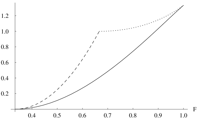
We consider the case of two qutrits () separately as an illustration of what happens in the general qudit case. Of the three extrema, , , and , we already know that the minimum is given by , i.e., , . This fact can also be seen from Fig. 1, where we have plotted the three extrema.

To calculate , it is necessary to analyze the behavior of . In Fig. 2, we plot the first and second derivatives of . The first derivative confirms that is monotonically increasing. The second derivative changes sign from positive to negative; changes from convex to concave where the second derivative vanishes. The tangle is the largest convex function bounded above by , which is constructed in the following way. Find the (unique) line tangent to that passes through the point ; for smaller than the tangent point, the tangle is given by , but for larger than the tangent point, the tangle is given by the line. The tangent point is found by solving the equation , which gives . The slope of the line is , and the tangle at the tangent point is . Thus the tangle for is
| (46) |
This function is plotted in Fig. 3.

The behavior of means that the pure states in an optimal ensemble decomposition for the tangle all have the same tangle for , but have two values of tangle, and (maximal entanglement), for .
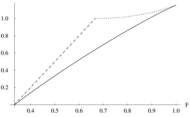
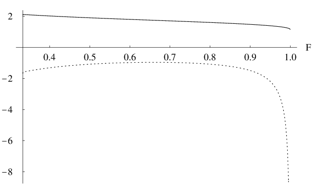
Of the three extrema for the concurrence, , , and , the minimum is given by , a fact confirmed by the plots in Fig. 4. In contrast to the situation with the tangle, however, the second derivative of is always negative (see Fig. 5), which means that is concave. Therefore the qutrit concurrence is the straight line passing through the points and , i.e.,
| (47) |
The concavity of means that the pure states in an optimal ensemble decomposition for the concurrence are either product states or maximally entangled states.
III.4.3 Two qudits
For arbitrary , we have already established that . It turns out that for arbitrary , has the same behavior as for ; i.e., it changes from convex to concave as increases. We get at this behavior by calculating the second derivative of from Eq. (44):
| (48) |
Notice that for this expression simplifies to , as it should. For , the polynomial in large parentheses in Eq. (48) clearly has one root for positive ; it is easy to verify that this one root occurs in the range of interest, i.e., between () and (), showing that changes from convex to concave as increases.
We find the tangle just as for , i.e., by finding the line tangent to that passes through the point . Solving the equation gives a tangent point at , where the tangle and slope are and . Thus the tangle is given by
| (49) |
The tangle is plotted for a few representative values of in Fig. 3. The pure states in an optimal ensemble decomposition for the tangle all have the same tangle for , but have two values of tangle, and (maximal entanglement), for . As , becomes a linear function.
The concurrence also has the same behavior generally as for . A calculation of using Eqs. (44) and (48) shows that is a concave function on the range of interest. Thus the concurrence of isotropic states is a linear function between zero concurrence at the separability boundary and maximal entanglement at :
| (50) |
The pure states in an optimal ensemble decomposition for the concurrence are either product states or maximally entangled states. As , .
IV Conclusion
It is informative to conclude the paper by comparing our results for the tangle of isotropic states with the results of Terhal and Vollbrecht Terhal2000 for the entanglement of formation.
If one follows through the procedure of Terhal and Vollbrecht Terhal2000 for finding the entanglement of formation, one finds that the function is replaced by the function
| (51) |
where and is the binary entropy function. The entanglement of formation, , is given by the largest convex function that is bounded above by . Terhal and Vollbrecht conjecture that has the properties that we find here for , i.e., that has a single inflection point in the range , changing from convex to concave as increases. Given this conjecture, the entanglement of formation is found by finding the straight line tangent to that passes through the point . Remarkably the tangent point for is the same as for , which gives the entanglement of formation as
| (52) |
Asymptotically, as , the entanglement of formation becomes . The similarity of the tangle and entanglement of formation must reflect a deep connection between the two, at least for isotropic states, but we have not been able to find a simple reason for this similarity.
Acknowledgements.
This work was supported in part by Office of Naval Research Contract No. N00014-00-1-0578.References
- (1) A. Einstein, B. Podolski, and N. Rosen, Phys. Rev. 47, 777 (1935).
- (2) J. S. Bell, Physics 1, 195 (1964).
- (3) W. K. Wootters, Quant Inf. Comp. 1, 27 (2001).
- (4) Introduction to Quantum Computation and Information, edited by H.-K. Lo, S. Popescu, and T. Spiller (World Scientific, Singapore, 1998).
- (5) M. A. Nielsen and I. L. Chuang, Quantum Computation and Quantum Information (Cambridge University Press, Cambridge, England, 2000).
- (6) C. H. Bennett, H. J. Bernstein, S. Popescu, and B. Schumacher, Phys. Rev. A 53, 2046 (1996).
- (7) C. H. Bennett, D. P. DiVincenzo, J. A. Smolin, and W. K. Wootters, Phys. Rev. A 54, 3824 (1996).
- (8) V. Vedral and M. B. Plenio, Phys. Rev. A 57, 1619 (1996).
- (9) V. Vedral, Rev. Mod. Phys. 74, 197 (2002).
- (10) G. Vidal and R. Tarrach, Phys. Rev. A 59, 141 (1999).
- (11) S. Hill and W. K. Wootters, Phys. Rev. Lett. 78, 5022 (1997).
- (12) W. K. Wootters, Phys. Rev. Lett. 80, 2245 (1998).
- (13) P. Rungta, V. Bužek, C. M. Caves, M. Hillery, and G. J. Milburn, Phys. Rev. A 64, 042315 (2001).
- (14) G. Vidal, J. Mod. Opt. 47, 355 (2000).
- (15) G. Vidal, Phys. Rev. Lett. 83, 1046 (1999).
- (16) S. Popescu and D. Rohrlich, Phys. Rev. A 56, R3319 (1997).
- (17) P. Hayden, M. Horodecki, and B. M. Terhal, J. Phys. A 34, 6891 (2001).
- (18) M. A. Nielsen, Phys. Rev. A 61, 064301 (2000).
- (19) M. A. Nielsen, Phys. Rev. Lett. 83, 436 (1999).
- (20) D. Jonathan and M. B. Plenio, Phys. Rev. Lett. 83, 1455 (1999).
- (21) G. Vidal and D. Jonathan and M. A. Nielsen, Phys. Rev. A 62, 012304 (2000).
- (22) V. Coffman, J. Kundu, and W. K. Wootters, Phys. Rev. A 61, 052306 (2000).
- (23) T. J. Osborne, unpublished, arXiv.org e-print quant-ph/0203087.
- (24) B. M. Terhal and K. G. H. Vollbrect, Phys. Rev. Lett. 85, 2625 (2000).
- (25) A. Wehrl, Rev. Mod. Phys. 50, 221 (1978).
- (26) P. Rungta, W. J. Munro, K. Nemoto, P. Deuar, G. J. Milburn, and C. M. Caves, in Directions in Quantum Optics: A Collection of Papers Dedicated to the Memory of Dan Walls, edited by H. J. Carmichael, R. J. Glauber, and M. O. Scully (Springer, Berlin, 2001), p. 149.
- (27) M. Horodecki and P. Horodecki, Phys. Rev. A 59, 4206 (1999).