The Magnetic Casimir Effect

Since its discovery, the Casimir effect has gradually become a much-discussed subject in physics. Originally, one understood by the Casimir effect the attractive force between two metal plates in vacuum as a result of zero-point quantum fluctuations HBGCas. Nowadays the term is used for a much broader range of effects, all involving the influence of boundaries on fluctuations. As such, the Casimir effect plays a role in quantum field theory, atomic and molecular physics, condensed matter physics, gravitation, cosmology and so on. A thorough review of the Casimir effect in all these fields was published recently MBor.

For two uniformly magnetized ferromagnetic plates held parallel to each other, it is shown in a previous paper PBru that the interplay of the Casimir effect and the magneto-optical Kerr effect gives rise to a new long-range magnetic interaction. In [PBru], this magnetic Casimir force was found to decay with interplate distance D as $D^{-5}$ in the limit of long distances, and as $D^{-1}$ for short distances. In this case, the ferromagnetic plates were described with a Drude model and the magnetization was defined to be perpendicular to the plates. In view of future experimental investigations of this new magnetic Casimir force, it would be useful to study the case where the magnetization is parallel to the plates since this situation is easier to obtain in an experimental setup. This subject will be studied in the present paper and a force which decays as $D^{-6}$ in the long-distance limit and as $D^{-3}$ in the limit of short distances is found when the Drude model is used. This behavior is interesting since it means that the force is larger, and thus easier to measure, for in-plane magnetization than for perpendicular magnetization at sufficiently small distances. Next to the Drude model, another more realistic model is also studied. In this so called hybrid model, a plasma model is used for the diagonal element of the dielectric tensor of the magnetic plates, and a single absorption line model for the off-diagonal element. As for the long distance limit, the force in this model goes like $D^{-8}$ for the case of perpendicular magnetization and as $D^{-10}$ when the magnetization is parallel to the plates while the behavior in the short-distance limit is unchanged. Finally we will present some numerical calculations of the interaction for Fe, in which experimental data for the elements of the dielectric tensor are used. An experimental setup to measure the magnetic Casimir force is also discussed.

Consider two uniformly magnetized ferromagnetic plates of infinite lateral extension held parallel to each other. The Casimir interaction energy per unit area at $T=0$ between the plates can be expressed as MTJae:

$${\cal E}=\frac{\hbar}{(2\pi)^{3}}\int_{0}^{+\infty}{\rm d}\omega\int\,{\rm d}^{2}\bm{k}_{\parallel}\,\mbox{Im Tr}\ln(1-{\sf R}_{A}{\sf R}_{B}{\rm e}^{2{\rm i}k_{\perp}D}),$$

(1)

where $k_{\perp}$ and $\bm{k}_{\parallel}$ are the components of the wavevector perpendicular and parallel to the mirrors. The $2\times 2$ matrices ${\sf R}_{A}$ and ${\sf R}_{B}$ contain the reflection coefficients of the two mirrors:

$${\sf R}_{A(B)}=\left(\begin{array}[]{cc}r_{ss}^{A(B)}&r_{sp}^{A(B)}\\ r_{ps}^{A(B)}&r_{pp}^{A(B)}\end{array}\right)$$

(2)

The index $s$ (resp. $p$) corresponds to a polarization with the electric field perpendicular (resp. parallel) to the incidence plane. We will adopt here the usual convention that the $s$ axis remains unchanged upon reflection. Since the reflection coefficients are dependent on the direction of the magnetisation of the mirrors, it is clear from Eqs. (1) and  (2) that the magnetic Casimir energy between the mirrors will differ for the situations in which the magnetizations of the two mirrors are parallel (FM) or antiparallel (AF). This will result in a net magnetic Casimir force per unit area $\Delta{\cal F}\equiv{\cal F}_{AF}-{\cal F}_{FM}$ between the mirrors, different from the ordinary Casimir force discussed in Ref. [HBGCas].
If a change of integration variables $(\omega,\bm{k}_{\parallel})\longrightarrow(\omega,k_{\perp},\varphi)$ is performed and complex integration methods are used as in [MTJae], Eq. (1) can be written as:

$${\cal E}=\frac{\hbar}{(2\pi)^{3}}\int_{0}^{+\infty}{\rm d}k_{\perp}\,k_{\perp}\int_{0}^{2\pi}{\rm d}\varphi\int_{0}^{k_{\perp}c}{\rm d}\omega\,\mbox{Re Tr}\ln[1-{\sf R}_{A}({\rm i}\omega,{\rm i}k_{\perp},\varphi){\sf R}_{B}({\rm i}\omega,{\rm i}k_{\perp},\varphi){\rm e}^{-2k_{\perp}D}]$$

(3)

In general, the reflection coefficients contain terms of different orders of the magneto-optical constant Q. In our calculation, only terms up to first order in Q will be conserved. When the magnetisation direction is reversed, these terms will change sign. Since the first order terms are usually much smaller than 1 and than the terms that are independent of Q, it is possible to expand expression (3) to lowest order in the linear terms.

Consider two identical magnetic mirrors with a dielectric tensor described by the Drude model:

	$\displaystyle\varepsilon_{xx}({\rm i}\omega)$	$\displaystyle=$	$\displaystyle 1+\frac{\omega_{p}^{2}\tau}{\omega(1+\omega\tau)},$		(8a)
	$\displaystyle\varepsilon_{xy}({\rm i}\omega)$	$\displaystyle=$	$\displaystyle\frac{\omega_{p}^{2}\omega_{c}\tau^{2}}{\omega(1+\omega\tau)^{2}}.$		(8b)

In this equation $\omega_{p}$ is the plasma frequency defined by $\omega_{p}\equiv 4\pi ne^{2}/m^{\star}$; $\omega_{c}$ is the cyclotron frequency given by $\omega_{c}\equiv eB_{{\rm eff}}/m^{\star}c$ where $B_{{\rm eff}}$ is the effective magnetic field experienced by the conduction electrons as a result of exchange and spin-orbit interactions; $\tau$ is the relaxation time. In the usual situation: $\omega_{c}\tau\ll 1\ll\omega_{p}\tau$.

There are three important distance regimes to consider. In the long distance limit ($D\gg c\tau$) the dominant part in the integrals in Eqs. (4) and (6) comes from the region $\omega\leq k_{\perp}c\approx c/D\ll 1/\tau$. In this range, one has:

	$\displaystyle\varepsilon_{xx}({\rm i}\omega)$	$\displaystyle\approx$	$\displaystyle\varepsilon_{xx}({\rm i}\omega)-1\approx\frac{\omega_{p}^{2}\tau}{\omega}\gg 1,$		(9a)
	$\displaystyle\varepsilon_{xy}({\rm i}\omega)$	$\displaystyle\approx$	$\displaystyle\frac{\omega_{p}^{2}\omega_{c}\tau^{2}}{\omega}.$		(9b)

With these approximations, one finds for the reflection coefficients:

	$\displaystyle r_{ss}({\rm i}\omega,{\rm i}k_{\perp})$	$\displaystyle\approx$	$\displaystyle-r_{pp}({\rm i}\omega,{\rm i}k_{\perp})\approx-1,$		(10a)
	$\displaystyle r_{sp}^{\perp}({\rm i}\omega,{\rm i}k_{\perp})$	$\displaystyle\approx$	$\displaystyle-\frac{\omega_{c}}{\omega_{p}}\sqrt{\omega\tau},$		(10b)
	$\displaystyle r_{sp}^{\parallel}({\rm i}\omega,{\rm i}k_{\perp})$	$\displaystyle\approx$	$\displaystyle-\frac{\omega_{c}}{\omega_{p}^{2}}\sqrt{\omega^{2}-(k_{\perp}c)^{2}},$		(10c)
	$\displaystyle\Delta r_{pp}({\rm i}\omega,{\rm i}k_{\perp})$	$\displaystyle\approx$	$\displaystyle\frac{2\omega_{c}}{\omega_{p}^{2}}\,\frac{\omega\sqrt{\omega^{2}-(k_{\perp}c)^{2}}}{k_{\perp}c},$		(10d)

For the polar configuration, we arrive at:

	$\displaystyle\Delta{\cal E}^{\perp}$	$\displaystyle\approx$	$\displaystyle-\frac{3\zeta(3)}{16\pi^{2}}\,\frac{{\omega_{c}}^{2}\tau}{{\omega_{p}}^{2}}\,\frac{\hbar c^{2}}{D^{4}},$		(11a)
	$\displaystyle\Delta{\cal F}^{\perp}$	$\displaystyle\approx$	$\displaystyle-\frac{3\zeta(3)}{4\pi^{2}}\,\frac{{\omega_{c}}^{2}\tau}{{\omega_{p}}^{2}}\,\frac{\hbar c^{2}}{D^{5}},$		(11b)

While for the in-plane configuration it is found that:

	$\displaystyle\Delta{\cal E}_{1}^{\parallel}$	$\displaystyle\approx$	$\displaystyle-\frac{\zeta(4)}{4\pi^{2}}\frac{\omega_{c}^{2}}{\omega_{p}^{4}}\,\frac{\hbar c^{3}}{D^{5}},\ \Delta{\cal E}_{2}^{\parallel}\approx\frac{\zeta(4)}{10\pi^{2}}\frac{\omega_{c}^{2}}{\omega_{p}^{4}}\,\frac{\hbar c^{3}}{D^{5}},$		(12a)
	$\displaystyle\Delta{\cal E}^{\parallel}$	$\displaystyle=$	$\displaystyle\Delta{\cal E}_{1}^{\parallel}+\Delta{\cal E}_{2}^{\parallel}\approx-\frac{3\zeta(4)}{20\pi^{2}}\,\frac{\omega_{c}^{2}}{\omega_{p}^{4}}\,\frac{\hbar c^{3}}{D^{5}},$		(12b)
	$\displaystyle\Delta{\cal F}_{1}^{\parallel}$	$\displaystyle\approx$	$\displaystyle-\frac{5\zeta(4)}{4\pi^{2}}\frac{\omega_{c}^{2}}{\omega_{p}^{4}}\,\frac{\hbar c^{3}}{D^{6}},\ \Delta{\cal F}_{2}^{\parallel}\approx\frac{\zeta(4)}{2\pi^{2}}\frac{\omega_{c}^{2}}{\omega_{p}^{4}}\,\frac{\hbar c^{3}}{D^{6}},\ \$		(12c)
	$\displaystyle\Delta{\cal F}^{\parallel}$	$\displaystyle=$	$\displaystyle\Delta{\cal F}_{1}^{\parallel}+\Delta{\cal F}_{2}^{\parallel}\approx-\frac{3\zeta(4)}{4\pi^{2}}\,\frac{\omega_{c}^{2}}{\omega_{p}^{4}}\,\frac{\hbar c^{3}}{D^{6}}.$		(12d)

The second regime is that for intermediate distances ($c/\omega_{p}\ll D\ll c\tau$). Now the integrals in Eqs. (4) and (6) are dominated by the range $1/\tau\ll\omega\leq k_{\bot}c\approx c/D\ll\omega_{p}$. For the elements of the dielectric tensor one then finds:

	$\displaystyle\varepsilon_{xx}({\rm i}\omega)$	$\displaystyle\approx$	$\displaystyle\varepsilon_{xx}({\rm i}\omega)-1\approx\frac{{\omega_{p}}^{2}}{\omega^{2}}\gg 1,$		(13a)
	$\displaystyle\varepsilon_{xy}({\rm i}\omega)$	$\displaystyle\approx$	$\displaystyle\frac{{\omega_{p}}^{2}\omega_{c}}{\omega^{3}}.$		(13b)

In this case, the reflection coefficients $r_{ss}$, $r_{pp}$, $r_{sp}^{\parallel}$ and $\Delta r_{pp}$ still satisfy Eqs. (10a-10d), while

$$r_{sp}^{\perp}\approx-\frac{\omega_{c}}{\omega_{p}}.$$

(14)

Since the reflection coefficients for the in-plane configuration in this regime are not different from the ones in the short distance limit, the expressions (12) are still valid for the Casimir magnetic energies and forces in the in-plane configuration. However, for the polar configuration, one has:

	$\displaystyle\Delta{\cal E}^{\perp}$	$\displaystyle\approx$	$\displaystyle-\,\frac{1}{24}\,\frac{\hbar c}{D^{3}}\,\frac{{\omega_{c}}^{2}}{{\omega_{p}}^{2}},$		(15a)
	$\displaystyle\Delta{\cal F}^{\perp}$	$\displaystyle\approx$	$\displaystyle-\,\frac{1}{8}\,\frac{\hbar c}{D^{4}}\,\frac{{\omega_{c}}^{2}}{{\omega_{p}}^{2}}.$		(15b)

The third regime to be considered is the limit of short distances ($D\ll c/\omega_{p}$). Here one has to distinguish between two regions: (i) $\omega\leq k_{\bot}c\ll\omega_{p}$ and (ii) $\omega_{p}\ll\omega\leq k_{\bot}c$. In region (i) the dielectric tensor elements are given in Eqs. (13), so the reflection coefficients $r_{sp}^{\perp}$, $r_{sp}^{\parallel}$ and $\Delta r_{pp}$ are the same as those in the intermediate distance regime, but we will now make an expansion for $r_{ss}$ and $r_{pp}$ around $-1$ and $1$ respectively:

$$r_{ss}({\rm i}\omega,{\rm i}k_{\perp})\approx-1+\frac{2k_{\perp}c}{\omega_{p}},\ \ \ r_{pp}({\rm i}\omega,{\rm i}k_{\perp})\approx 1-2\frac{\omega^{2}}{\omega_{p}k_{\perp}c}$$

(16)

In region (ii) the dielectric tensor elements are given by:

	$\displaystyle\varepsilon_{xx}({\rm i}\omega)-1$	$\displaystyle\approx$	$\displaystyle\frac{\omega_{p}^{2}}{\omega^{2}}\ll 1,$		(17a)
	$\displaystyle\varepsilon_{xy}({\rm i}\omega)$	$\displaystyle\approx$	$\displaystyle\frac{\omega_{p}^{2}\omega_{c}}{\omega^{3}}.$		(17b)

We then find for region (ii):

	$\displaystyle r_{ss}({\rm i}\omega,{\rm i}k_{\perp})$	$\displaystyle\approx$	$\displaystyle 0,\ r_{pp}({\rm i}\omega,{\rm i}k_{\perp})\approx\frac{\omega_{p}^{2}}{2\omega^{2}+\omega_{p}^{2}},\ \ \ \ \ \$		(18a)
	$\displaystyle r_{sp}^{\perp}({\rm i}\omega,{\rm i}k_{\perp})$	$\displaystyle\approx$	$\displaystyle-\frac{{\omega_{p}}^{2}\omega_{c}}{2}\,\frac{1}{(k_{\perp}c)(2\omega^{2}+{\omega_{p}}^{2})},$		(18b)
	$\displaystyle r_{sp}^{\parallel}({\rm i}\omega,{\rm i}k_{\perp})$	$\displaystyle\approx$	$\displaystyle-\frac{\omega_{p}^{2}\omega_{c}}{2}\,\frac{\sqrt{\omega^{2}-(k_{\perp}c)^{2}}}{(k_{\perp}c)^{2}(2\omega^{2}+\omega_{p}^{2})},$		(18c)
	$\displaystyle\Delta r_{pp}({\rm i}\omega,{\rm i}k_{\perp})$	$\displaystyle\approx$	$\displaystyle 2\omega_{p}^{2}\omega_{c}\,\frac{\omega\sqrt{\omega^{2}-(k_{\perp}c)^{2}}}{(k_{\perp}c)(2\omega^{2}+\omega_{p}^{2})^{2}}.$		(18d)

With these approximations for the reflection coefficients in regions (i) and (ii), one finds the following expressions for the energies and forces (only the dominant term is given):

	$\displaystyle\Delta{\cal E}^{\perp}$	$\displaystyle\approx$	$\displaystyle-\frac{1}{16\sqrt{2}\pi}\,\omega_{c}^{2}\sqrt{\omega_{p}}\,\frac{\hbar}{c^{3/2}D^{1/2}},$		(19a)
	$\displaystyle\Delta{\cal F}^{\perp}$	$\displaystyle\approx$	$\displaystyle-\frac{1}{32\sqrt{2}\pi}\,\omega_{c}^{2}\sqrt{\omega_{p}}\,\frac{\hbar}{c^{3/2}D^{3/2}},$		(19b)
	$\displaystyle\Delta{\cal E}_{1}^{\parallel}$	$\displaystyle\approx$	$\displaystyle-\frac{1}{96\sqrt{2}\pi}\,\omega_{c}^{2}\sqrt{\omega_{p}}\,\frac{\hbar}{c^{3/2}D^{1/2}},$		(19c)
	$\displaystyle\Delta{\cal F}_{1}^{\parallel}$	$\displaystyle\approx$	$\displaystyle-\frac{1}{192\sqrt{2}\pi}\,\omega_{c}^{2}\sqrt{\omega_{p}}\,\frac{\hbar}{c^{3/2}D^{3/2}},$		(19d)
	$\displaystyle\Delta{\cal E}_{2}^{\parallel}$	$\displaystyle\approx$	$\displaystyle\frac{1}{16\sqrt{2}\pi}\sum_{n=0}^{+\infty}\left[\frac{(4n+3)!!}{(n+1)(4n+6)!!}\right]\frac{\omega_{c}^{2}}{\omega_{p}}\frac{\hbar}{D^{2}},\ \ \ \$		(19e)
	$\displaystyle\Delta{\cal F}_{2}^{\parallel}$	$\displaystyle\approx$	$\displaystyle\frac{1}{8\sqrt{2}\pi}\sum_{n=0}^{+\infty}\left[\frac{(4n+3)!!}{(n+1)(4n+6)!!}\right]\frac{\omega_{c}^{2}}{\omega_{p}}\frac{\hbar}{D^{3}},\ \ .$		(19f)

From these expressions, it is obvious that $\Delta{\cal E}^{\parallel}\approx\Delta{\cal E}_{2}^{\parallel}$ and $\Delta{\cal F}^{\parallel}\approx\Delta{\cal F}_{2}^{\parallel}$ for distances small enough. Note that for the polar configuration, the exponent of the dependence with respect to D obtained here in the short distance limit differs from the one obtained in Ref. [PBru]. This is due to the effect of multiple reflections, which were neglected in Ref. [PBru] in this regime. It is interesting to note that although the reflection coefficients are much smaller than 1 in this high-frequency limit, the effect of multiple reflections is so important that the analytical dependence with D is modified. This is a unique feature of the magnetic Casimir effect.
It is clear that in the polar configuration, the energies are always negative. For the in-plane configuration however, $\Delta{\cal E}_{2}^{\parallel}$ is positive, while $\Delta{\cal E}_{1}^{\parallel}$ is negative, so the sign of the resulting energy $\Delta{\cal E}^{\parallel}=\Delta{\cal E}_{1}^{\parallel}+\Delta{\cal E}_{2}^{\parallel}$ will depend on the magnitude of these two terms in the different regimes. As a result, a change of sign of the interaction is observed; in the long and intermediate distance regimes, the total energy $\Delta{\cal E}^{\parallel}$ is negative, while for short distances it is positive. So whether the magnetic Casimir interaction is negative or positive depends on the distance between the mirrors.
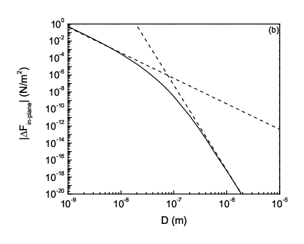
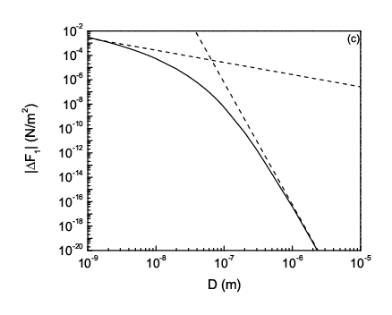
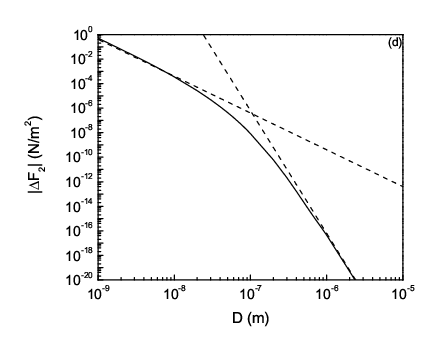
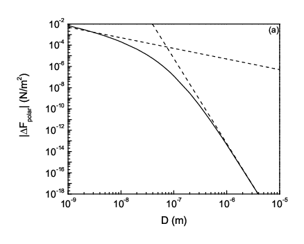
We numerically calculated Eqs. (4) and (6) and compared them to the analytical expressions derived above. Details of the numerical procedure will be given in section V. The absolute values of the magnetic Casimir forces per unit area (both numerical and analytical results) for distances between 1 nm and 10 $\mu$m for the two configurations are plotted in Fig. 1. Since typically $\tau\approx 10^{-13}$ s, the long distance regime ($D\gg c\tau\approx 10\ \mu$m) will not be visible in these plots. For the plots, a Drude model is used with $\hbar\omega_{c}=5.9$ meV and $\hbar\omega_{p}=9.85$ eV. As expected from the analytical results, the force in the in-plane configuration will be larger than that for the polar configuration for small enough distances ($D<10$ nm). The discontinuity at $D\approx 40$ nm in the plot of the in-plane case depicts the change of sign. The analytical results are in pretty good agreement with the numerical calculations.

The Drude model is not very realistic. Although it describes rather well the diagonal part of the dielectric tensor (except of course for the effect of interband transitions, which are not very important here), the off-diagonal part of the dielectric tensor is poorly described. This is because the latter is dominated by interband transitions. We therefore introduce a model (called “hybrid model”) in which $\varepsilon_{xx}$ is described by a plasma model,

$$\varepsilon_{xx}({\rm i}\omega)=1+\frac{\omega_{p}^{2}}{\omega^{2}},$$

(20)

and where $\varepsilon_{xy}$ is described by a single absorption line interband transition:

$$\mbox{Re }\varepsilon_{xy}(\omega)\approx\omega_{0}\,\varepsilon_{xy}^{\rm eff}\,\delta(\omega-\omega_{0}).$$

(21)

In real systems $\omega_{0}$ will be of the same order of magnitude as $\omega_{p}$. The off-diagonal element of the dielectric tensor at imaginary frequency can be obtained by the following Kramers-Krönig relation:

$$\varepsilon_{xy}({\rm i}\omega)=\frac{2}{\omega\pi}\int_{0}^{+\infty}\!\!\!{\rm d}\omega^{\prime}\,\frac{{\omega^{\prime}}^{2}\,\mbox{ Re }\varepsilon_{xy}(\omega^{\prime})}{{\omega^{\prime}}^{2}+\omega^{2}},$$

(22)

and in this way we arrive at:

$$\varepsilon_{xy}({\rm i}\omega)=\frac{2}{\pi}\,\frac{\omega_{0}^{3}\,\varepsilon_{xy}^{\rm eff}}{\omega(\omega_{0}^{2}+\omega^{2})}.$$

(23)

For this model, we will only have two different integration regimes; the long distance ($D\gg c/\omega_{p}$) and the short distance regime ($D\ll c/\omega_{p}$). In the long distance regime, the integrals in Eqs. (4) and (6) will be dominated by the range $\omega\leq k_{\perp}c\ll\omega_{p}$. In this range, we can approximate the dielectric tensor by:

	$\displaystyle\varepsilon_{xx}({\rm i}\omega)$	$\displaystyle\approx$	$\displaystyle\varepsilon_{xx}({\rm i}\omega)-1\approx\frac{\omega_{p}^{2}}{\omega^{2}}\gg 1,$		(24a)
	$\displaystyle\varepsilon_{xy}({\rm i}\omega)$	$\displaystyle\approx$	$\displaystyle\frac{2}{\pi}\,\frac{\omega_{0}\,\varepsilon_{xy}^{\rm eff}}{\omega}.$		(24b)

One then finds for the reflection coefficients:

	$\displaystyle r_{ss}({\rm i}\omega,{\rm i}k_{\perp})$	$\displaystyle\approx$	$\displaystyle-1,\ \ r_{pp}({\rm i}\omega,{\rm i}k_{\perp})\approx 1,$		(25a)
	$\displaystyle r_{sp}^{\perp}({\rm i}\omega,{\rm i}k_{\perp})$	$\displaystyle\approx$	$\displaystyle-\frac{2}{\pi}\,\frac{\omega_{0}\,\varepsilon_{xy}^{\rm eff}}{\omega_{p}^{3}}\omega^{2},$		(25b)
	$\displaystyle r_{sp}^{\parallel}({\rm i}\omega,{\rm i}k_{\perp})$	$\displaystyle\approx$	$\displaystyle-\frac{2}{\pi}\,\frac{\omega_{0}\,\varepsilon_{xy}^{\rm eff}}{\omega_{p}^{4}}\sqrt{\omega^{2}-(k_{\perp}c)^{2}}\,\omega^{2},$		(25c)
	$\displaystyle\Delta r_{pp}({\rm i}\omega,{\rm i}k_{\perp})$	$\displaystyle\approx$	$\displaystyle\frac{4}{\pi}\,\frac{\omega_{0}\,\varepsilon_{xy}^{\rm eff}}{\omega_{p}^{4}}\,\frac{\sqrt{\omega^{2}-(k_{\perp}c)^{2}}\,\omega^{3}}{k_{\perp}c}.$		(25d)

With these approximations, we obtain for the magnetic Casimir energies and forces (per unit area):

	$\displaystyle\Delta{\cal E}^{\perp}$	$\displaystyle\approx$	$\displaystyle-\frac{\pi^{2}}{210}\,\frac{\omega_{0}^{2}(\varepsilon_{xy}^{\rm eff})^{2}}{\omega_{p}^{6}}\,\frac{\hbar c^{5}}{D^{7}},$		(26a)
	$\displaystyle\Delta{\cal F}^{\perp}$	$\displaystyle\approx$	$\displaystyle-\frac{\pi^{2}}{30}\,\frac{\omega_{0}^{2}(\varepsilon_{xy}^{\rm eff})^{2}}{\omega_{p}^{6}}\,\frac{\hbar c^{5}}{D^{8}},$		(26b)
	$\displaystyle\Delta{\cal E}_{1}^{\parallel}$	$\displaystyle\approx$	$\displaystyle-\frac{\pi^{4}}{1050}\,\frac{\omega_{0}^{2}(\varepsilon_{xy}^{\rm eff})^{2}}{\omega_{p}^{8}}\,\frac{\hbar c^{7}}{D^{9}},$		(26c)
	$\displaystyle\Delta{\cal F}_{1}^{\parallel}$	$\displaystyle\approx$	$\displaystyle-\frac{9\pi^{4}}{1050}\,\frac{\omega_{0}^{2}(\varepsilon_{xy}^{\rm eff})^{2}}{\omega_{p}^{8}}\,\frac{\hbar c^{7}}{D^{10}},$		(26d)
	$\displaystyle\Delta{\cal E}_{2}^{\parallel}$	$\displaystyle\approx$	$\displaystyle\frac{\pi^{4}}{945}\,\frac{\omega_{0}^{2}(\varepsilon_{xy}^{\rm eff})^{2}}{\omega_{p}^{8}}\,\frac{\hbar c^{7}}{D^{9}},$		(26e)
	$\displaystyle\Delta{\cal F}_{2}^{\parallel}$	$\displaystyle\approx$	$\displaystyle\frac{\pi^{4}}{105}\,\frac{\omega_{0}^{2}(\varepsilon_{xy}^{\rm eff})^{2}}{\omega_{p}^{8}}\,\frac{\hbar c^{7}}{D^{10}},$		(26f)
	$\displaystyle\Delta{\cal E}^{\parallel}$	$\displaystyle\approx$	$\displaystyle\frac{\pi^{4}}{9450}\,\frac{\omega_{0}^{2}(\varepsilon_{xy}^{\rm eff})^{2}}{\omega_{p}^{8}}\,\frac{\hbar c^{7}}{D^{9}},$		(26g)
	$\displaystyle\Delta{\cal F}^{\parallel}$	$\displaystyle\approx$	$\displaystyle\frac{\pi^{4}}{1050}\,\frac{\omega_{0}^{2}(\varepsilon_{xy}^{\rm eff})^{2}}{\omega_{p}^{8}}\,\frac{\hbar c^{7}}{D^{10}}.$		(26h)

As in the Drude model, the force in the polar configuration will be negative. However, the total force for the in-plane configuration will be positive for the hybrid model in this distance regime.
In the limit of short distances, one has to distinguish between three different integration ranges while performing the integrals in Eqs. (4) and (6): region (i) where $\omega\leq k_{\perp}c\ll\omega_{p}$, region (ii) $k_{\perp}c\gg\omega_{p},\ \omega\ll\omega_{p}$ and region (iii) $k_{\perp}c\gg\omega_{p},\ \omega\gg\omega_{p}$. In region (i), $r_{ss}$ and $r_{pp}$ are defined by Eq. (16), while $r_{sp}^{\perp},\ r_{sp}^{\parallel}$ and $\Delta r_{pp}$ are given by Eqs. (25b-25d). In regions (ii) and (iii), we will do the calculations without multiple reflections (i.e., we put $r_{ss}({\rm i}\omega,{\rm i}k_{\perp})=r_{pp}({\rm i}\omega,{\rm i}k_{\perp})\approx 0$). In region (ii), the dielectric tensor elements are given in Eqs. (24), and the magneto-optical reflection coefficients are given by:

	$\displaystyle r_{sp}^{\perp}({\rm i}\omega,{\rm i}k_{\perp})$	$\displaystyle\approx$	$\displaystyle-\frac{1}{\pi}\,\omega_{0}\,\varepsilon_{xy}^{\rm eff}\,\frac{\omega^{2}}{(k_{\perp}c)(2\omega^{2}+\omega_{p}^{2})},$
	$\displaystyle r_{sp}^{\parallel}({\rm i}\omega,{\rm i}k_{\perp})$	$\displaystyle\approx$	$\displaystyle-\frac{1}{\pi}\,\omega_{0}\,\varepsilon_{xy}^{\rm eff}\,\frac{\sqrt{\omega^{2}-(k_{\perp}c)^{2}}\,\omega^{2}}{(k_{\perp}c)^{2}(2\omega^{2}+\omega_{p}^{2})},$
	$\displaystyle\Delta r_{pp}({\rm i}\omega,{\rm i}k_{\perp})$	$\displaystyle\approx$	$\displaystyle\frac{4}{\pi}\,\omega_{0}\,\varepsilon_{xy}^{\rm eff}\,\frac{\sqrt{\omega^{2}-(k_{\perp}c)^{2}}\,\omega^{3}}{(k_{\perp}c)(2\omega^{2}+\omega_{p}^{2})^{2}}.$

In region (iii), the dielectric tensor can be approximated by:

	$\displaystyle\varepsilon_{xx}({\rm i}\omega)-1$	$\displaystyle\approx$	$\displaystyle\frac{\omega_{p}^{2}}{\omega^{2}}\ll 1,$		(28a)
	$\displaystyle\varepsilon_{xy}({\rm i}\omega)$	$\displaystyle\approx$	$\displaystyle\frac{2}{\pi}\,\frac{\omega_{0}^{3}\,\varepsilon_{xy}^{\rm eff}}{\omega^{3}}.$		(28b)

One then finds for the magneto-optical reflection coefficients in region (iii):

	$\displaystyle r_{sp}^{\perp}({\rm i}\omega,{\rm i}k_{\perp})$	$\displaystyle\approx$	$\displaystyle-\frac{1}{\pi}\,\omega_{0}^{3}\,\varepsilon_{xy}^{\rm eff}\,\frac{1}{(k_{\perp}c)(2\omega^{2}+\omega_{p}^{2})},$
	$\displaystyle r_{sp}^{\parallel}({\rm i}\omega,{\rm i}k_{\perp})$	$\displaystyle\approx$	$\displaystyle-\frac{1}{\pi}\,\omega_{0}^{3}\,\varepsilon_{xy}^{\rm eff}\,\frac{\sqrt{\omega^{2}-(k_{\perp}c)^{2}}}{(k_{\perp}c)^{2}(2\omega^{2}+\omega_{p}^{2})},$
	$\displaystyle\Delta r_{pp}({\rm i}\omega,{\rm i}k_{\perp})$	$\displaystyle\approx$	$\displaystyle\frac{4}{\pi}\,\omega_{0}^{3}\,\varepsilon_{xy}^{\rm eff}\,\frac{\sqrt{\omega^{2}-(k_{\perp}c)^{2}}\,\omega}{(k_{\perp}c)(2\omega^{2}+\omega_{p}^{2})^{2}}.$

With these equations by hand, we made an interpolation for the reflection coefficients in region (ii) and (iii). This makes the calculation of the integrals less labor-intensive because we can calculate the two regions at the same time. We have put:

	$\displaystyle r_{sp}^{\perp}({\rm i}\omega,{\rm i}k_{\perp})$	$\displaystyle\approx$	$\displaystyle-\frac{\omega_{0}^{3}\,\varepsilon_{xy}^{\rm eff}}{\pi}\,\frac{\omega^{2}}{(k_{\perp}c)(2\omega^{2}+\omega_{p}^{2})(\omega^{2}+\omega_{0}^{2})},$		(30a)
	$\displaystyle r_{sp}^{\parallel}({\rm i}\omega,{\rm i}k_{\perp})$	$\displaystyle\approx$	$\displaystyle-\frac{\omega_{0}^{3}\,\varepsilon_{xy}^{\rm eff}}{\pi}\,\frac{\sqrt{\omega^{2}-k_{\perp}c^{2}}\,\omega^{2}}{(k_{\perp}c)^{2}(2\omega^{2}+\omega_{p}^{2})(\omega^{2}+\omega_{0}^{2})},$		(30b)
	$\displaystyle\Delta r_{pp}({\rm i}\omega,{\rm i}k_{\perp})$	$\displaystyle\approx$	$\displaystyle\frac{4\omega_{0}^{3}\,\varepsilon_{xy}^{\rm eff}}{\pi}\,\frac{\sqrt{\omega^{2}-(k_{\perp}c)^{2}}\,\omega^{3}}{(k_{\perp}c)(2\omega^{2}+\omega_{p}^{2})^{2}(\omega^{2}+\omega_{0}^{2})}.$		(30c)

With these expressions for the reflection coefficients, we are finally ready to calculate the magnetic Casimir energies and forces for the short distance regime. The result is:

	$\displaystyle\Delta{\cal E}^{\perp}$	$\displaystyle\approx$	$\displaystyle-\frac{1}{4\sqrt{2}\pi^{3}}\,\frac{\omega_{0}^{6}(\varepsilon_{xy}^{\rm eff})^{2}}{(\omega_{p}+\sqrt{2}\omega_{0})^{3}}\,\frac{\hbar}{c^{2}}\ln\left(\frac{c}{\omega^{\star}D}\right),\ \ \ \ \$		(31a)
	$\displaystyle\Delta{\cal F}^{\perp}$	$\displaystyle\approx$	$\displaystyle-\frac{1}{4\sqrt{2}\pi^{3}}\,\frac{\omega_{0}^{6}(\varepsilon_{xy}^{\rm eff})^{2}}{(\omega_{p}+\sqrt{2}\omega_{0})^{3}}\,\frac{\hbar}{c^{2}D},$		(31b)
	$\displaystyle\Delta{\cal E}_{1}^{\parallel}$	$\displaystyle\approx$	$\displaystyle-\frac{1}{8\sqrt{2}\pi^{3}}\,\frac{\omega_{0}^{6}(\varepsilon_{xy}^{\rm eff})^{2}}{(\omega_{p}+\sqrt{2}\omega_{0})^{3}}\,\frac{\hbar}{c^{2}}\ln\left(\frac{c}{\omega^{\star}D}\right),$		(31c)
	$\displaystyle\Delta{\cal F}_{1}^{\parallel}$	$\displaystyle\approx$	$\displaystyle-\frac{1}{8\sqrt{2}\pi^{3}}\,\frac{\omega_{0}^{6}(\varepsilon_{xy}^{\rm eff})^{2}}{(\omega_{p}+\sqrt{2}\omega_{0})^{3}}\,\frac{\hbar}{c^{2}D},$		(31d)
	$\displaystyle\Delta{\cal E}_{2}^{\parallel}$	$\displaystyle\approx$	$\displaystyle\frac{1}{64\sqrt{2}\pi^{3}}\,\frac{\omega_{0}^{6}(\varepsilon_{xy}^{\rm eff})^{2}(\omega_{p}+5\sqrt{2}\omega_{0})}{\omega_{p}(\omega_{p}+\sqrt{2}\omega_{0})^{5}}\,\frac{\hbar}{D^{2}},$		(31e)
	$\displaystyle\Delta{\cal F}_{2}^{\parallel}$	$\displaystyle\approx$	$\displaystyle\frac{1}{32\sqrt{2}\pi^{3}}\,\frac{\omega_{0}^{6}(\varepsilon_{xy}^{\rm eff})^{2}(\omega_{p}+5\sqrt{2}\omega_{0})}{\omega_{p}(\omega_{p}+\sqrt{2}\omega_{0})^{5}}\,\frac{\hbar}{D^{3}},\ \ \$		(31f)

with $\omega^{\star}$ a cut-off frequency of the order of the plasma frequency $\omega_{p}$. It is clear that $\Delta{\cal E}^{\parallel}\approx\Delta{\cal E}_{2}^{\parallel}$ and $\Delta{\cal F}^{\parallel}\approx\Delta{\cal F}_{2}^{\parallel}$ for distances small enough. The force for the in-plane configuration is positive in this short distance regime too, so there will not be a change of sign for this model.
We did the same numerical calculations as for the Drude model and compared the results with the analytical expressions in the different regimes. The following parameters were used in our hybrid model: $\hbar\omega_{p}=9.85$ eV, $\hbar\omega_{0}=3.9$ eV, $\varepsilon_{xy}^{\rm eff}=1.5\ 10^{-2}$ and we have put $\omega^{\star}=2\,\exp(1)\,\omega_{p}$. In Fig. 2 the numerical and analytical results for the absolute value of the magnetic Casimir force are shown to be in rather good agreement.

References

• (1) H.B.G. Casimir, Proc. K. Ned. Akad. Wet. 51, 793 (1948).
• (2) M. Bordag, U. Mohideen, and V.M. Mostepanenko, Phys. Rep. 353, 1 (2001).
• (3) P. Bruno, Phys. Rev. Lett. 88, 240401 (2002).
• (4) M.T. Jaekel and S. Reynaud, J. Physique I 1, 1395 (1991).
• (5) G. Metzger, P. Pluvinage, and R. Torguet, Ann. Phys. Fr. 10, 5 (1965).
• (6) S.K. Lamoreaux, Phys. Rev. A 59, 3149 (1999).
• (7) A. Lambrecht and S. Reynaud, Eur. Phys. J. D 8, 309 (2000).
• (8) Handbook of Optical Constants of Solids, edited by E.D. Palik (Academic Press, New York, 1991).
• (9) Landolt-Boernstein, Numerical Data and Functional Relationships in Science and Technology, New Series III/19a (Springer, Berlin, 1992).
• (10) U. Mohideen and A. Roy, Phys. Rev. Lett. 81, 4549 (1998).
• (11) A.  Roy, C.-Y. Lin, and U. Mohideen, Phys. Rev. D 60, 111101(R) (1999).
• (12) B.W. Harris, F. Chen, and U. Mohideen, Phys. Rev. A 62, 052109 (2000).
• (13) J. Blocki, J. Randrup, W.J. Swiatecki, and C.F. Tsang, Ann. Phys. 105, 427 (1977).
• (14) D. Rugar, O. Züger, S. Hoen, C.S. Yannoni, H.-M. Vieth, and R.D. Kendrick, Science 264, 1560 (1994).
• (15) J.A. Sidles, J.L. Garbini, K.J. Bruland, D. Rugar, O. Züger, S. Hoen, and C.S. Yannoni, Rev. Mod. Phys. 67, 249 (1995).
• (16) T.D. Stowe, K. Yasumura, T.W. Kenny, D. Botkin, K. Wago, and D. Rugar, Appl. Phys. Lett. 71, 288 (1997).
• (17) P. Mohanty, D.A. Harrington, and M.L. Roukes, Physica B 284-288, 2143 (2000).
• (18) A. Roy and U. Mohideen, Phys. Rev. Lett. 82, 4380 (1999).